At Hubbard Decision Research, we’ve built dozens upon dozens of risk models for companies of different sizes across wildly diverse areas. One of the questions we sometimes get from the more quantitatively affluent clients is “Should we use a power law distribution or a lognormal distribution to model the impact of this risk?”. On the surface, it seems like a simple question. However, when you’re dealing with highly uncertain ranges for some impacts, the question gets a bit more complicated. Ultimately, the choice comes down to a few key components: Identifying which approach best fits your data, understanding the uncertainties regarding growth and tail behavior, as well as existing assumptions regarding a specific impact (such as the natural limit of the impact or how the impact scales).
Both power law distributions and log normal distributions are relatively common in quantitative risk modeling. They have some similarities because neither can result in a zero or negative value in a simulation and both have larger positive tails (which is very important in capturing ranges of impacts). However, the difference between them can drastically alter decisions if you’re not careful. Choosing a lognormal distribution when the data really fits a power law would result in you underestimating your losses by potentially astronomical amounts. Choosing a power law when the data really fits a lognormal could result in overprioritizing smaller risks when they were not really justified. Both of these scenarios are not ideal and having the flexibility to accurately fit your data to the correct distribution is essential for prioritizing mitigations or controls (especially large portfolios of mitigations/controls).
How do you choose which to use? There are a few approaches to this, and the most noticeable differences live in the tail of the distributions. A power law distribution assumes that these extreme events happen more often than a lognormal does. If your business decisions depend on how, you treat these rare events, this difference can have a big impact. If you’re worried about a few massive events driving most of your losses, and your data suggests there’s no natural limit to how bad things can get, the power law might be the better fit compared to a lognormal distribution. On the other hand, if you’re modeling something that tends to grow or spread gradually, like cost overruns or delays, with a known limit for about how bad losses/impacts can be, the lognormal could be more realistic alternative.

One of the key differences to understand is how each distribution handles growth. A lognormal distribution assumes a steady, compounding process, like many small risks building up over time. For example, if you are modeling network risk, equipment ages and wears out over time. Those losses would likely accumulate steadily and fit a lognormal distribution. A power law, on the other hand, assumes a more chaotic buildup, where both the size and number of risks can grow unpredictably. In our network risk example, this might be reflected best in large internet outages or application outages which are triggered by uncertain yet cascading failures. So, while lognormal reflects consistent compounding, power law reflects compounding under deep uncertainty.
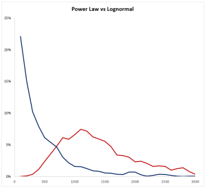
The best-case scenario is to use the data you have available to compare which distribution fits best. Also, there is a lot of historical precedence for the use of certain distributions so don’t fly solo if you don’t have to. An axiom we have at HDR is that it has probably been measured before. Look at what others have done and the rationale for why they have done so as you make your choice. Risk modeling isn’t about being perfect, it’s about improving upon the existing approach. If you’re currently using qualitative or pseudo-quantitative approaches like scales or scores, either option will probably move you in a better direction. On the book website (linked at the bottom) you can find a spreadsheet that goes with Appendix A where you can input elements to generate both lognormal distributions and power law distributions. I encourage you to experiment with these and familiarize yourself with the characteristics of these distributions. In Figure 1, I used a simple simulation with 1000 trials comparing monetary losses using a Lomax power law and a lognormal distribution which have the same average which highlights the need to understand the general trends of the data, as well as the assumptions outlined earlier.

Figure 1: Simulation Output Power Law vs. Lognormal with the Same Mean
Don’t let perfect be the enemy of good (to quote Voltaire). However, recognize when and where different distributions can and should be used. If this is something you’re having trouble with, HDR helps clients with this on a daily basis. Measure what matters, make better decisions, and keep moving in the right direction.


