The Cost of Being Late: What Businesses Can Learn from Successful F1 Teams

The Cost of Being Late: What Businesses Can Learn from Successful F1 Teams

I have been a Formula 1 fan, and a motorsport fan in general, for as long as I can remember. Some of my favorite childhood moments were spent watching drivers like Damon Hill and Mika Häkkinen go to battle with Michael Schumacher. As I got older, the data and strategy elements of F1 became more and more fascinating as I learned about statistics, probability, and analytics. Over time, I started to realize that F1 teams were just applying the same methods to solve their unique problems and optimize their decisions. This in itself isn’t shocking, but to a student at university, it was eye-opening. When managers collect reports and review dashboards, it should be for the purpose of informing decisions.  If there is no intention or ability to act on this information, its value is zero.  But do they know what specific decisions they are trying to inform?  Do they know the combinations of all the data they read that should inform a specific action at a specific time?  Often, they rely on hope.  They hope that among all the data they receive they will detect when action is needed.  They hope they will choose the right action based on accurate forecasts of outcomes based on that data.  But a manager doesn’t have to rely on their ability to detect what may be subtle movements in several data sources, run forecasts in their heads, and make subjective judgements based on that.  Some decision makers know that the consequences of delayed and poor-quality decisions are unacceptable.   Formula racing, for example, has a solution for making well thought out decisions based on dozens of rapidly changing variables in tight time constraints.

F1 teams have to make decisions under uncertainty, just like any other organization. For example, determining the optimal tire strategy is fundamental in order to maximize a team’s result in a race. The consequences of these decisions are massive, not only from the sporting side but also from the financial side. Whether the outcome of a decision impacts winning a race, a world championship, or scraping the last points position in a Grand Prix, there is substantial consequence.

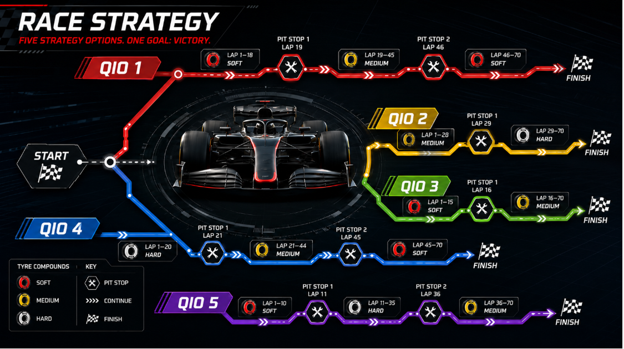
Optimizing these decisions relies on the use of quantitative intervention options, or QIOs. QIOs are predefined interventions based on signals in data. They are tied to thresholds where action needs to be taken. Delays in taking action, or acting too early, can result in suboptimal performance. In F1, that can cost teams points or victories. In other organizations, similar delays can cost millions of dollars.

Staying with our tire strategy example, strategy engineers and data teams constantly wade through millions of data points trying to find the ideal conditions that prompt a driver to pit. The ocean of data is continuously tracked and fed into decision models that run simulations to determine the optimum strategy given the information available. The weather, tire temperature and pressure, engine temperatures, lap time, including sector time and mini-sector time, fuel levels, tire wear information from observing other teams, and feedback from the driver are all examples of factors being considered and acted upon in real time. Pulling the trigger at the right time requires clearly defined QIOs, which are thoroughly discussed during team strategy meetings. These QIOs can result in large lists of strategy options to consider depending on what happens during a race. You often hear Ferrari team radios where the race engineer says, “We are on plan C,” for example. That means the strategy team has observed a pattern in the data that suggests a QIO is needed to optimize the race result. In fact, work by Thomas and colleagues (2025) demonstrated improvements based upon QIOs can be optimized using reinforcement learning showing how specific strategy optimization can improve finishing position (I reference the article at the end of the post).

In F1, you’ll often see a team react a fraction late to another team’s optimal strategy, and that can cost a team or driver a win or valuable points. It can be a game of fine margins. The same thing is true for critical business decisions surrounding projects. In Doug’s latest book, How to Measure Anything in Project Management, the signals for canceling a project were present well before the plug was pulled. Canceling a project late, or not pivoting early, can have a huge cost. According to work done by Oxford Global Projects, less than 1% of projects, from a sample of over 16,000, finish on time, on budget, and with the expected benefits, meaning many of these projects should have had QIOs to avoid costly delays or better identify the conditions in which a project needs to be canceled.

One of the most common objections we get when starting out on projects or from individuals taking our training is that we don’t have all of the variables. Neither do F1 teams. They can’t foresee everything, but they have processes in place that allow them to be nimble and take action using what information they have to optimize the outcome, even when crazy stuff happens over a race weekend. During a race, you’ll often hear a race engineer tell a driver a lap target, then say “plus 5,” or another value, to communicate that the tire strategy is the same, but they are going to go longer on the initial set of tires than initially anticipated based upon the updated data the team has. This could be because there is traffic that the car would come out into behind them, the tire wear was less than they had anticipated at normal racing speed, or they spent time behind a safety car, which extended the life of the tires. Again, this holds true in the business world. No model, quantitative or otherwise, has every single variable mapped out. Despite this, having a quantitative model in place allows for options to be tested and conditions for QIOs to be monitored and optimized. In the paper I cited earlier, the simulated improvements when QIOs were being implemented based upon models, the improvements were pronounced. Finishing positions noticeably improved without any mechanical or aerodynamic changes. This highlights how improved process and utilization of data, quantitative interventions, and planning can drastically improve outcomes.

Going from having no quantitative decision model to an F1-level solution doesn’t happen overnight, nor should it. HDR recommends an iterative approach centered around the decisions that matter to your organization that follows Doug’s Applied Information Economics (AIE) framework. AIE is a practical collection of methods designed to optimize efficiency by identifying what variables actually need to be measured or monitored for a particular decision. See Figure 1 for a diagram about the AIE framework.

Step 1: Define your decision or decisions.

This sounds simple, but in order to create decision-driven dashboards, you need at least one clearly defined decision. This could be which vendor to use for a project, whether to hire additional resources, or whether to cancel a project. In F1, one decision could be whether the car should pit to replace a damaged front wing.

Step 2: Model your current state of uncertainty.

You do not need to boil the ocean in your model from the beginning. You want to leverage well-informed calibrated estimates, or easily accessible information, to start with. Modeling what you know now saves time and resources later. Many of the variables organizations spend time measuring have no influence on actual decisions and end up wasting time. For the F1 front wing example, you might estimate a range of time loss given the damage and include that uncertainty in a model.

Step 3: Determine the value of additional information.

The monetary value of measuring each variable in a model can be computed by determining the value of information, or VOI. VOI helps prioritize resources by identifying the variables that can actually influence your decision. As mentioned in Step 2, many of the variables organizations routinely measure have little to no impact on the decisions they actually care about. By computing information value, you can measure what actually matters. In the front wing example, this would mean determining the value of better information about the amount of time the car is expected to lose because of the damage.

Step 4: Measure high-value information.

As Doug wrote in his first book, How to Measure Anything: Finding the Value of Intangibles in Business, everything is measurable. Objections to this usually stem from a misunderstanding of the concept, object, or method of measurement. High-information-value variables are often easier to measure than lower-information-value variables because they are usually more uncertain. If a range for a given variable is wide, reducing that range does not require as much information as it would if the range were already narrow.

This step repeats as needed based on additional VOI calculations. For the front wing example, one quick measurement would be to evaluate several mini-sectors as the car is on its way back to the pits. The car has to drive there anyway, or retire from the race. If the mini-sectors show only a minimal loss of time, or if the team can evaluate the points of downforce lost and simulate the effect further, it might not be worth coming in to replace the wing. After a few mini-sectors, the uncertainty regarding time loss should be reduced enough to inform the QIO.

Step 5: Optimize the decision.

Take the information from the model and apply it to the actual decision. Rely on decision-driven dashboards to indicate what action should be taken. This does not take away from the expertise of the team. Rather, it reuses that expertise in a way that avoids many of the pitfalls of human judgment. Decisions with high consequences and complexity should not live inside an individual’s head. They should be explicitly and carefully modeled.

To conclude the damaged wing example, based on the reduced uncertainty from observations, the team would decide whether to replace the wing or continue racing as is, thereby optimizing its race given the damage to the car.

In summary, every organization makes complex decisions under uncertain conditions. To optimize those decisions and produce the best possible outcomes, even in the face of uncontrollable external events, organizations need a quantitative framework and predefined QIOs. Having those in place can change the trajectory of an organization. This applies to virtually every major project or business decision.

If you want to modernize your organization’s decision-making processes and develop decision-driven dashboards, contact Hubbard Decision Research using our Contact Us Page (Contact | Hubbard Decision Research). We have built models with QIOs in many industries including utilities, aerospace, manufacturing, consumer products, and many more. Whether you are a large firm or a family business, you have complicated decisions that have large consequences for your organization. Knowing how and when to act is a competitive advantage.
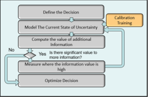
Figure 1 AIE Framework

References:

Thomas, D., Jiang, J., Kori, A., Russo, A., Winkler, S., Sale, S., … & Rago, A. (2025, March). Explainable reinforcement learning for Formula One race strategy. In Proceedings of the 40th ACM/SIGAPP Symposium on Applied Computing (pp. 1090-1097).

 

Power Law vs. Lognormal Distribution: Which is the Right Choice for My Model?

Power Law vs. Lognormal Distribution: Which is the Right Choice for My Model?

At Hubbard Decision Research, we’ve built dozens upon dozens of risk models for companies of different sizes across wildly diverse areas. One of the questions we sometimes get from the more quantitatively affluent clients is “Should we use a power law distribution or a lognormal distribution to model the impact of this risk?”. On the surface, it seems like a simple question. However, when you’re dealing with highly uncertain ranges for some impacts, the question gets a bit more complicated. Ultimately, the choice comes down to a few key components: Identifying which approach best fits your data, understanding the uncertainties regarding growth and tail behavior, as well as existing assumptions regarding a specific impact (such as the natural limit of the impact or how the impact scales).

Both power law distributions and log normal distributions are relatively common in quantitative risk modeling. They have some similarities because neither can result in a zero or negative value in a simulation and both have larger positive tails (which is very important in capturing ranges of impacts). However, the difference between them can drastically alter decisions if you’re not careful. Choosing a lognormal distribution when the data really fits a power law would result in you underestimating your losses by potentially astronomical amounts. Choosing a power law when the data really fits a lognormal could result in overprioritizing smaller risks when they were not really justified. Both of these scenarios are not ideal and having the flexibility to accurately fit your data to the correct distribution is essential for prioritizing mitigations or controls (especially large portfolios of mitigations/controls).

How do you choose which to use? There are a few approaches to this, and the most noticeable differences live in the tail of the distributions. A power law distribution assumes that these extreme events happen more often than a lognormal does. If your business decisions depend on how, you treat these rare events, this difference can have a big impact. If you’re worried about a few massive events driving most of your losses, and your data suggests there’s no natural limit to how bad things can get, the power law might be the better fit compared to a lognormal distribution. On the other hand, if you’re modeling something that tends to grow or spread gradually, like cost overruns or delays, with a known limit for about how bad losses/impacts can be, the lognormal could be more realistic alternative.

One of the key differences to understand is how each distribution handles growth. A lognormal distribution assumes a steady, compounding process, like many small risks building up over time. For example, if you are modeling network risk, equipment ages and wears out over time. Those losses would likely accumulate steadily and fit a lognormal distribution.  A power law, on the other hand, assumes a more chaotic buildup, where both the size and number of risks can grow unpredictably. In our network risk example, this might be reflected best in large internet outages or application outages which are triggered by uncertain yet cascading failures. So, while lognormal reflects consistent compounding, power law reflects compounding under deep uncertainty.

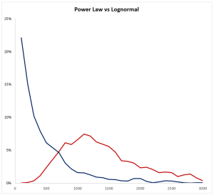
The best-case scenario is to use the data you have available to compare which distribution fits best. Also, there is a lot of historical precedence for the use of certain distributions so don’t fly solo if you don’t have to. An axiom we have at HDR is that it has probably been measured before. Look at what others have done and the rationale for why they have done so as you make your choice. Risk modeling isn’t about being perfect, it’s about improving upon the existing approach. If you’re currently using qualitative or pseudo-quantitative approaches like scales or scores, either option will probably move you in a better direction. On the book website (linked at the bottom) you can find a spreadsheet that goes with Appendix A where you can input elements to generate both lognormal distributions and power law distributions. I encourage you to experiment with these and familiarize yourself with the characteristics of these distributions. In Figure 1, I used a simple simulation with 1000 trials comparing monetary losses using a Lomax power law and a lognormal distribution which have the same average which highlights the need to understand the general trends of the data, as well as the assumptions outlined earlier.

Figure 1: Simulation Output Power Law vs. Lognormal with the Same Mean


Don’t let perfect be the enemy of good (to quote Voltaire). However, recognize when and where different distributions can and should be used. If this is something you’re having trouble with, HDR helps clients with this on a daily basis. Measure what matters, make better decisions, and keep moving in the right direction.

How To Measure Anything in Cybersecurity Risk | Downloads

Herd Immunity and State Health Departments

Herd Immunity and State Health Departments

Misallocation of Vaccines Leads to 75,000 Additional US Deaths…At Least

As we prepare to roll out the vaccine across the United States, we are faced with an unparalleled opportunity. But there is also a danger of squandering the opportunity. States will distinguish themselves by the speed with which they get their populations to herd immunity, and by the degree to which they minimize the number of people who die during the period when the vaccine is provided.

The number of vaccines available per month is outside of your control. Therefore, as a decision maker, the lever for affecting outcomes lies in your decisions about what order (and which of) your citizens get the vaccine. Certain populations should clearly be at the front of the line (e.g. health care workers without SARS COV2 antibodies). But many questions remain: does the benefit of knowing who has antibodies justify the cost of an antibody test? Should you prioritize people more likely to spread COVID (front-line workers) or people more vulnerable to adverse outcomes (comorbid/elderly).

Vaccination Strategies for Minimizing Deaths

How vaccines are distributed can make a huge difference in the duration of economic effects, hospitalizations, and even deaths.  Our analysis shows that nationwide an optimized distribution strategy is 90% likely to avoid more than 75,000 deaths over simpler distribution strategies. The same analysis shows that even for a medium sized state, improved vaccination strategies could reduce the duration of the pandemic by two months and could reduce the number of deaths due to COVID infection by more than 1,000 people.  

This is accomplished by how we make tradeoffs among three guiding principles: 

  1. Don’t vaccinate people who have already had the infection.
  2. Vaccinate people who are more likely to infect others.
  3. Vaccinate vulnerable people (elderly and people with comorbidities are at higher risk of dying.)

There is extensive research indicating likelihood of reinfection is low and that infection with SARS-COV2 confers long term immunity[1][2][3][4]. One might therefore think the lowest hanging fruit would be to prioritize immunizations for the population that does not have antibodies or memory T cells for SARS-COV2. Unfortunately, only 10-20% of those who have had the illness are “visible” as indicated by a confirmed COVID test[5]. The remaining 80-90% of the already immune population is indistinguishable from the people who are not immune. So which tool should you use to reveal who is in this “not immune” population – antibody tests or statistical analysis? The answer to this question is pivotal and will probably vary from county to county and city to city. What is your current strategy to answer this question?

The other pivotal question is whether a strategy will save more lives by focusing on vaccinating socially active [6] or by focusing on vaccinating vulnerable populations? It is relatively straightforward to determine who is in the most vulnerable population (elderly and people with comorbidities) but knowing which broad strategy saves more lives is not as clear.

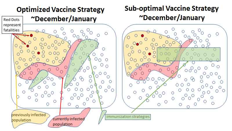
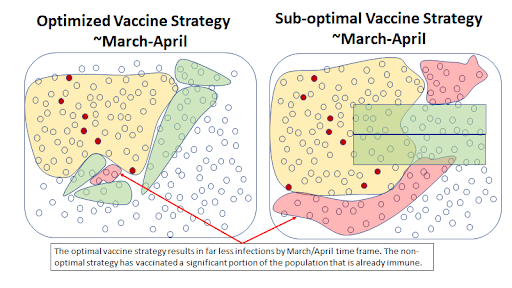
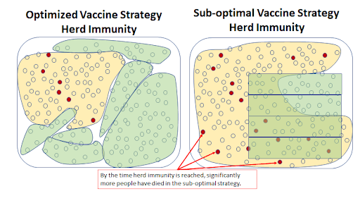
The charts below show how the virus may spread with an optimized strategy vs. a less effective strategy.  In the less effective strategy, some vaccines are wasted on individuals who already have antibodies.  In addition, the sub-optimal strategy would not attempt to identify recipients for the vaccine as a function of how likely they are to spread the virus to others.  

The better strategy minimizes the use of vaccines on people who do not need them and focuses on individuals more likely to spread the virus to others. Because this strategy slows down the rate of spread, it also allows more time to vaccinate the population not already immune.

The costs and benefits are also not limited to directly saving lives. Since the optimal strategy would also end community transmission more quickly, there would be economic benefits as well. For a medium sized state like Wisconsin, economic benefits would run in the billions of dollars (think opening a convention center 45 days before your neighboring states are able to do so). For the same state, the cost of getting the order wrong is a thousand or more (preventable) COVID deaths and a society shut down for 1 month+ longer than need be. As a decision maker for vaccine distribution, you get to decide whether to be seen as the hero…or the villain. But to be the hero, you need the right tools.

How Hubbard Decision Research Can Help

For 20+ years, Hubbard Decision Research has been “spreading the gospel” about probabilistic methods across many areas of industry and government. Probabilistic forecasting has been shown to yield the best results across all the industries where it has been measured and studied. We have the experience and expertise to bring these methods into any organization and any challenge. This year, HDR has also built a reputation for accurate forecasting and predictions with COVID related issues for businesses and municipalities, as well as national forecasting. We have presented webinars for the GFOA, and worked on COVID related operational risk projects for school districts, insurance and reinsurance companies, and a variety of other industries. Our Applied Information Economics methodology has been applied across industries, government, and the military and focuses on improving decisions through probabilistic modeling. 

Turn your vaccine distribution solution into an optimized quantitative solution. HDR offers a 20% discount on our rates for governments and nonprofits. Contact us to learn more.


[1]https://www.biorxiv.org/content/10.1101/2020.11.15.383323v1

[2] https://www.cell.com/immunity/pdf/S1074-7613(20)30312-5.pdf

[3] https://www.medrxiv.org/content/10.1101/2020.04.14.20065771v1.full.pdf

[4] https://www.nature.com/articles/s41586-020-2550-z?flip=true

[5] https://academic.oup.com/cid/advance-article/doi/10.1093/cid/ciaa1780/6000389

[6] N. Christakis, J. Fowler “Social Network Sensors for Early Detection of Contagious Outbreaks” PLoS One, 2010 e12948


Doug is Interviewed by Business Security Weekly

Doug is Interviewed by Business Security Weekly

Watch the interview with BSW that was previously aired on Tuesday, August 4th at 6:30pm CDT. Doug talks about his ground shaking exposé on the failure of popular cyber risk management methods, How To Measure Anything in Cybersecurity. This particular book is a Palo Alto Networks Cybersecurity Canon Award winner and the first of a series of spinoffs from his successful first book, How To Measure Anything: Finding the Value of “Intangibles” in Business. It is cited by the Center for Internet Security RAM Version 1.0 as a “thorough and practical guidance on using probability analysis for cybersecurity decision making.”

In the interview, Doug talks about his life’s work which is about building better “business impact” decision makers in any department of any sized organization and in any industry. He has sold over 150,000 copies of four different books in eight different languages. He offers powerful online training and consulting services revolving around his quantitative methodology, Applied Information Economics (AIE), for his global client base of Fortune 500 companies, federal and state governments, the United States military, and major non profits including the United Nations.

For this interview, Doug is particularly pleased with his shirt choice!  Enjoy!


Due to Popular Demand HDR Extends Offer on New AIE Analyst Series

Due to Popular Demand HDR Extends Offer on New AIE Analyst Series

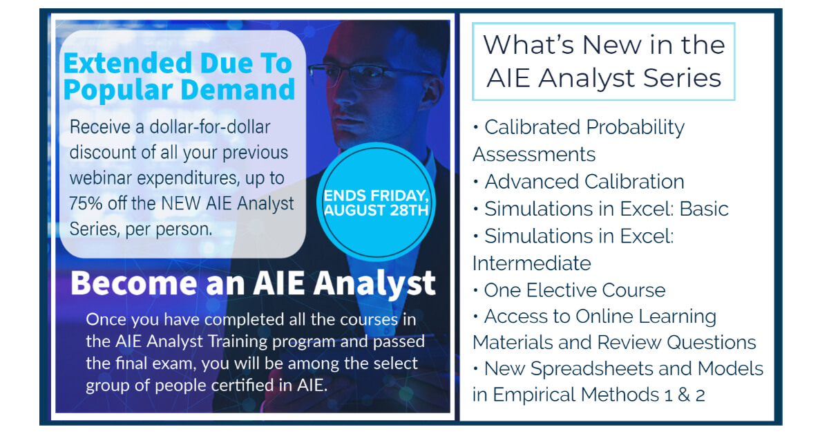
We heard you loud and clear and are happy to accommodate! We are extending our promotional offer on the NEW AIE Analyst Series through Friday, August 28th. Receive a dollar-for-dollar discount of all your previous webinar expenditures with HDR, up to 75% off the price of the new AIE Analyst Series, per person – if you book by Friday, August 28th.

The new AIE Analyst Series regular price is $1,950. This means you could take the entire series for as little as $487.50, if you have at least $1,462.50 in previous webinar expenditures. If you have more than $1,462.50 is previous webinar expenditures, invite a friend or colleague and (based on your remaining spend) they could also receive up to 75% off the series as well. This offer includes recordings of all courses in the series and access to online materials, even if you are unable to attend some or all of the live workshops.

Regular Prices on new courses included in the AIE Analyst Series:

  • Calibrated Probability Assessments – $580 (Pandemic Price: $325)
  • Advanced Calibration Methods – $995 (Pandemic Price: $550)
  • Creating Simulations in Excel: Basic – $375 (Pandemic Price: $310)
  • Creating Simulations in Excel: Intermediate – $375 (Pandemic Price: $310)
  • One Elective Course – $150 (Pandemic Price: $95)

(For Elective Course, Choose from: HTMA in Project Mgt, HTMA in Innovation, HTMA in Cybersecurity Risk, Failure of Risk Management)

Even courses that were part of the previous AIE Analyst series, such as Decisions Under Uncertainty and Empirical Measurements, have new methods and new spreadsheet tools.  And now the new Computer Based Training (CBT) components mean that you can review hours of content online at your own pace and take the review quizzes online.

If you have any questions or if you are interested to take advantage of this offer, please contact us at info@hubbardresearch.com to verify your previous webinar expenditures and to receive your unique promo code in order to claim your personalized discount at checkout.

Please click here to visit the AIE Analyst Series page of our website for more details and the date options for all courses included. 

Union Pacific CISO Gives a Shout Out to HDR’s AIE Framework

Union Pacific CISO Gives a Shout Out to HDR’s AIE Framework

Doug Hubbard and his team’s work is mentioned in high regard often in articles, by peers and clients alike. Perhaps it’s because HDR utilizes native Excel to create custom automation models for each client’s specific needs – without any limitations of an existing software solution and without annual licensing or subscription fees that often come along with traditional software solutions.

This week an article in InfoSec 2020 was brought to our attention where Doug is mentioned specifically by the Union Pacific CISO, Rick Holmes. Union Pacific is the second largest railroad system in the United States and is one of the largest transportation companies in the world.

A portion of the article reads, “UP assesses and analyzes risk from four different perspectives – those of an insurance company or actuarial expert, a compliance auditor, a legal advisor and the mind of an attacker. Key to the process, however, is the risk probability modeling that the cyber risk assessment team developed in order to statistically convey to upper management the likelihood of a cyber event occurring and the calculable monetary loss that would result.

For this, UP recruited management consultant and author Douglas Hubbard, who helped devise a framework that analyzed and categorized UP’s computing environment into various asset classes.”

Read the full article here.