Trojan Horse: How a Phenomenon Called Measurement Inversion Can Massively Cost Your Company

measurement inversion

Overview:

  • A Trojan horse is anything that introduces risk to an organization through something that appears to be positive
  • Measuring the wrong variables is a Trojan horse that infiltrates virtually every organization
  • This phenomenon has a real cost that can be measured – and avoided

The Trojans stood at the walls, drunk from victory celebrations after they had previously watched the Greek fleets set sail away in retreat, having been defeated after nearly 10 years of constant warfare. They had little reason to suspect treachery when they saw the massive wooden horse just outside their gates, apparently a gift offering from the defeated Greeks. Because of their confidence – or overconfidence – they opened the gates and claimed the wooden horse as the spoils of war.

Later that night, after the Trojans lay in drunken  stupor throughout the city, a force of Greek soldiers hidden in the horse emerged and opened the gates to the Greek army that had not retreated but had actually lay in wait just beyond sight of the city. Swords drawn and spears hefted, the Greek soldiers spread throughout the city and descended upon its people.

The end result is something any reader of The Illiad knows well: the inhabitants of Troy were slaughtered or sold into slavery, the city was razed to the ground, and the term “Trojan horse” became notorious for something deceitful and dangerous hiding as something innocuous and good.

Organizations are wising up to the fact that quantitative analysis is a vital part of making better decisions. Quantitative analysis can even seem like a gift, and used properly, it can be. However, the act of measuring and analyzing something can, in and of itself, introduce error – something Doug Hubbard calls the analysis placebo. Put another way, merely quantifying a concept and subjecting the data to an analytical process doesn’t mean you’re going to get better insights.

It’s not just what data you use, although that’s important. It’s not even how you make the measurements, which is also important. The easiest way to introduce error into your process is to measure the wrong things – and if you do, you’re bringing a Trojan horse into your decision-making.

Put another way, the problem is an insidious one: what you’re measuring may not matter at all, and may just be luring you into a false sense of security based on erroneous conclusions.

The One Phenomenon Every Quantitative Analyst Should Fear

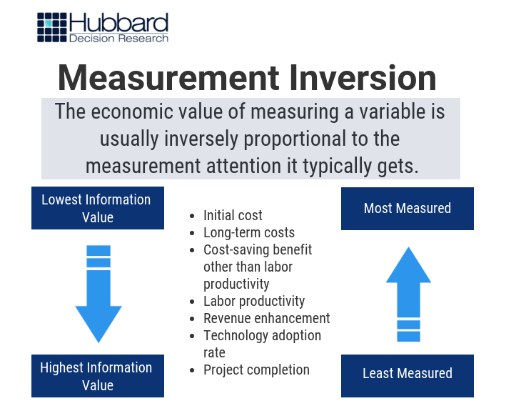
Over the past 20 years and throughout over 100 measurement projects, we’ve found a peculiar and pervasive phenomenon: that what organizations tend to measure the most often matters the least – and what they aren’t measuring tends to matter the most. This phenomenon is what we call measurement inversion, and it’s best demonstrated by the following image of a typical large software development project (Figure 1):

measurement problems

Figure 1: Measurement Inversion

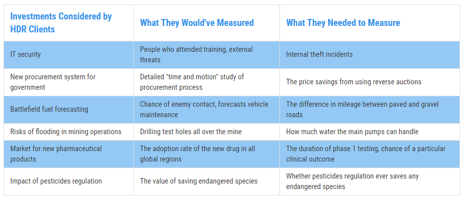
Some examples of measurement inversion we’ve discovered are shown below (Figure 2):

measurement inversion examples

Figure 2: Real Examples of Measurement Inversion

There are many reasons for measurement inversion, ranging from the innate inconsistency and overconfidence in subjective human assessment to organizational inertia where we measure what we’ve always measured, or what “best practices” say we should measure. Regardless of the reason, every decision-maker should know one, vital reality: measurement inversion can be incredibly costly.

Calculating the Cost of Measurement Inversion for Your Company

The Trojan horse cost Troy everything. That probably won’t be the case for your organization, as far as one measurement goes. But there is a cost to introducing error into your analysis process, and that cost can be calculated like anything else.

We uncover the value of each piece of information with a process appropriately named Value of Information Analysis (VIA). VIA is based on the simple yet profound premise that each thing we decide to measure comes with a cost and an expected value, just like the decisions these measurements are intended to inform. Put another way, as Doug says in How to Measure Anything, “Knowing the value of the measurement affects how we might measure something or even whether we need to measure it at all.” VIA is designed to determine this value, with the theory that choosing higher-value measurements should lead to higher-value decisions.

Over time, Doug has uncovered some surprising revelations using this method:

  • Most of the variables used in a typical model have an information value of zero
  • The variables with the highest information value were usually never measured
  • The most measured variables had low to no value.

The lower the information value of your variables, the less value you’ll generate from your model. But how does this translate into costs?

A model can calculate what we call your Overall Expected Opportunity Loss (EOL), or the average of each expected outcome that could happen as a result of your current decision, without measuring any further. We want to get the EOL as close to zero as possible. Each decision we make can either grow the EOL or shrink it. And each variable we measure can influence those decisions. Ergo, what we measure impacts our expected loss, for better or for worse.

If the variables you’re measuring have a low information value – or an information value of zero – you’ll waste resources measuring them and do little to nothing to reduce your EOL. The cost of error, then, is the difference between your EOL with these low-value variables and the EOL with more-valuable variables.

Case in point: Doug performed a VIA for an organization called CGIAR. You can read the full case study in How to Measure Anything, but the gist of the experience is this: by measuring the right variables, the model was able to reduce the EOL for a specific decision – in this case, a water management system – from $24 million to under $4 million. That’s a reduction of 85%.

Put another way, if they had measured the wrong variables, then they would’ve incurred a possible cost of $20 million, or 85% of the value of the decision.

The bottom line is simple. Measurement inversion comes with a real cost for your business, one that can be calculated. This raises important questions that every decision-maker needs to answer for every decision:

  1. Are we measuring the right things?
  2. How do we know if we are?
  3. What is the cost if we aren’t?

If you can answer these questions, and get on the right path toward better quantitative analysis, you can be more like the victorious Greeks – and less like the citizens of a city that no longer exists, all because what they thought was a gift was the terrible vehicle of their destruction. 


Learn how to start measuring variables the right way – and create better outcomes – with our hybrid learning course, How To Measure Anything: Principles of Applied Information Economics.


I am concerned about the CI, median and normal distribution

Originally posted at http://www.howtomeasureanything.com, on Wednesday, February 11, 2009 2:16:38 PM, by andrey.

“Hello Douglas,

First of all let me say I have thoroughly enjoyed reading your book. I have a technical background (software engineering) and have always been surprised at how “irresponsible” some business-level decision making can be – based on gut instincts and who-knows-what. This ‘intuitive’ approach is plagued with biases and heuristics, the effects of such approach has been widely publicized (for example here). This is one of many reasons I found your book very simulating and the AIE approach as a whole very promising.

However I have reservations about a few points you make. Please forgive me my ignorance if my questions are silly, my math has become rusty with the years passing by.

One of my concerns is the validity of the assumption that you make when explaining ‘The Rule of Five’, 90% CI and especially when using Monte Carlo simulation. I can believe (although it would’ve been great to see the sources) that ‘there is a 93% chance that the median of a population is between the smallest and largest values in any random sample of five from that population’. But when you are applying this to the Monte Carlo simulations, you assume that the mean (which is also the median for symmetric probability distributions) is exactly in the middle of the confidence interval. Which, I think, makes a big difference to the outcome because of the shape of the normal distribution function. If you assume the the median is for example very close to the lower or upper bound of the confidence interval by putting a different value into the =norminv(rand(),A, B) formula the results would be different.

I am still working through your book (second reading), trying to ‘digest’ and internalise it properly. I would be very grateful if you could explain this to me.

Thank you very much,

Andrey”

Thanks for your comment.

I don’t show a source (I’m the one who coined the term “Rule of Five” in this context) but I show the simple calculation, which is easily verifiable. The chance of randomly picking one sample with a parameter value above the true population median for that parameter is, by definition, 50%. We ask “what is the probability that I could happen to randomly choose five samples in a row that are all above the true population median?” It is the same chance as flipping five coins and getting all heads. The answer is 1/2^5 or 3.125% Likewise, the probability that we could have just picked 5 in a row that were all below the true population median is 3.125%. That means that there is a 93.75% chance that some were above and some were below – in other words, that the median is really between the min and max values in the sample. It’s not an “assumption” at all – it is a logically necessary conclusion from the meaning of the word “median”.

You can verify this experimentally as well. Try generating any large set of continuous values you like using any distribution you like (or just define a distribution function for such a set). Determine the median for the set. Then randomly select 5 from the set and see if the known population median is between the min and max values of those 5 samples. Repeat this a large number of times. You will find that 93.75% of the time the known median will be between the min and max values of the sample of 5.

I believe I also made it clear that this only applies to the median and not the mean. I further stated that if, on the other hand, you were able to make the determination that the distribution is symmetrical then, of course, it applies to the mean as well. Often, you may have reason to do this and this is no different than the assumption in any application of a t-stat or z-stat based calculation of a CI (which are always assumed to be symmetrical).

Furthermore, you certainly should not use a function that generates a normally distributed random number if you know it not to be normally distributed and I don’t believe I recommended otherwise. If you know the median and the mean of the distribution you intend to generate are not the same, then you can’t count on Excel’s normdist function to be a good approximation. For the sake of simplicity, I gave a very limited set of distributions functions for random values in Excel. But we can certainly add a lot more (triangular, beta, lognormal, etc.)

My approach is not to assume anything you don’t have to. If you don’t know that the distribution isn’t lopsided, you can simulate that uncertainty, too. Is it possible that the real distribution could actually be lognormal? Then put a probability on that and generate accordingly. Why “assume” something is true if we can explicitly model that we are uncertain about something?

Thanks,

Doug

Computing the Value of Information

 Originally posted at http://www.howtomeasureanything.com, on Monday, December 08, 2008 10:08:08 PM, by Unknown.

“I’m trying to quickly identify the items I need to spend time measuring. In your book, you determine what to measure by computing the value of information. You refer to a macro that you run on your spreadsheet that automatically computes the value of information and thus permits you to identify those items most worth spending extra time to refine their measurements. Once I list potential things that I might want to measure, do I estimate, using my Calibrated Estimators, a range for the chance of being wrong and the cost of being wrong and using something like @RISK, multiply these two lists of probability distributions together to arrive at a list of distributions for all the things I might want to measure? Then, do I look over this list of values of information and select the few that have significantly higher values of information?

I don’t want you to reveal your proprietary macro, but am I on the right track to determining what the value of information is?”

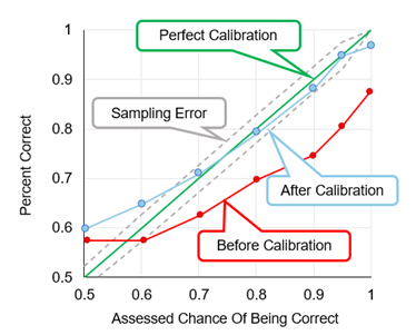
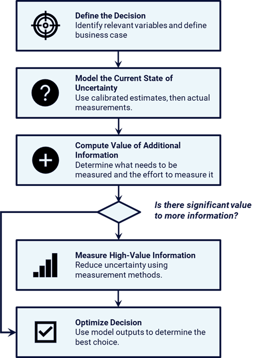
You were on track right up to the sentence that starts Once I list potential things that I might want to measure. You already have calibrated estimates by that point. Remember, you have to have calibrated estimates first before you even can compute the value of information. Once the value of information indicates that you need to measure something, then its time to get new observations. As I mention in the book, you could also use calibrated estimates for this second round, but only if you are giving them new information that will allow them to reduce their uncertainty.

So, first you have your original calibrated estimates, THEN you compute the value of information, THEN you measure the things that matter. In addition to using calibrated estimators again (assuming you are finding new data to give them to reduce their ranges) I mention several methods in the book including decomposition, sampling methods, controlled experiments, and several other items. It just depends on what you need to measure.

Also, the chance of being wrong and the cost of being wrong can already be computed from the original calibrated estimates you provided and the business case you put them in. You do not have to estimate them separately in addition to the original calibrated estimates themselves. Look at the examples I gave in the chapter on the value of information.

My macros make it more convenient to more complicated information values, but they are not necessary for the simplest examples. Did you see how I computed the information values in that chapter? I already had calibrated estimates on the measurements themselves. Try a particular example and ask me about that example specifically if you are still having problems.

Thanks for your use of my book and please stay in touch.

Doug Hubbard