The Role of Calibration in Risk Analysis

The Role of Calibration in Risk Analysis

HDR’s Calibration Training: Team Calibrator – Hubbard Decision Research

Managing risk requires making decisions under uncertainty, often before complete information is available. One of the most common objections we encounter when working with clients concerns the lack of data to inform quantitative model inputs. When data are easily accessible, leveraging them to generate empirical inputs is straightforward. Gaps still arise, however, or data collection becomes impractical, especially early in a project. Under such conditions, we rely on “calibrated estimates” from subject matter experts (SMEs).

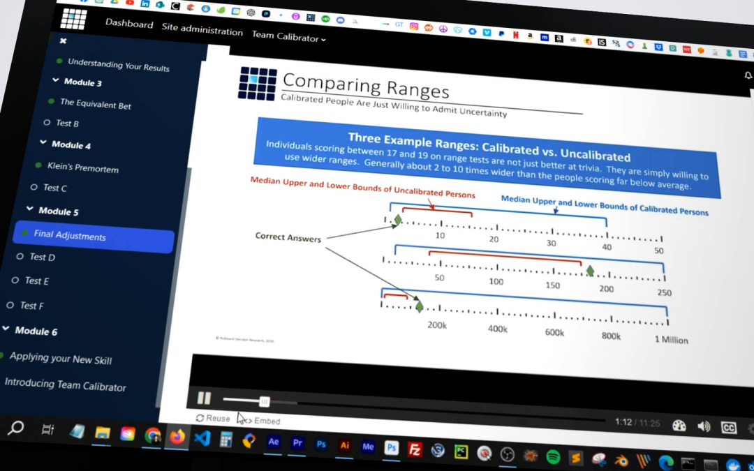
Every measurement instrument requires calibration, whether the instrument involves a precision manufacturing tool or human judgment used in model building. Calibration depends on consistent and unambiguous feedback. Prior to calibration, measurement error is often quite large. Humans tend to be systematically overconfident when making estimates, which introduces error and reduces model realism. Such overconfidence appears both in 90% confidence-interval range estimates and in probability estimates for binary events.

In training more than 3,000 individuals through consulting engagements and standalone programs, HDR has repeatedly observed this pattern of overconfidence. Calibration exercises demonstrably improve performance. Our methods, along with those developed by Philip Tetlock and Roger Cooke—whose pioneering work in this field is well worth reading—align stated confidence with empirical accuracy. Calibration in this context means that a claim of 90% confidence in a range estimate corresponds, across repeated estimates, to correctness approximately 90% of the time within a statistically allowable error range.

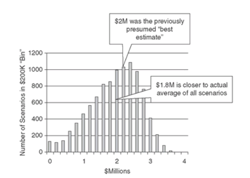
Figure 1 illustrates the typical pattern observed for calibration improvement over time. Despite systematic improvement, several confidence levels remain difficult for aggregated groups to calibrate perfectly. Slight overconfidence commonly appears when individuals state 50% confidence in a binary event. Such statements suggest complete uncertainty, yet outcomes across many trials indicate the presence of some informational advantage. Slight overconfidence also appears near the 100% confidence level, where allowable error approaches zero. To address these residual effects, estimates are aggregated across multiple experts and adjusted using each expert’s observed calibration performance. Aggregation reduces individual bias, and final calibration adjustments further fine-tune estimates, producing more reliable inputs for decision models.

Figure 1


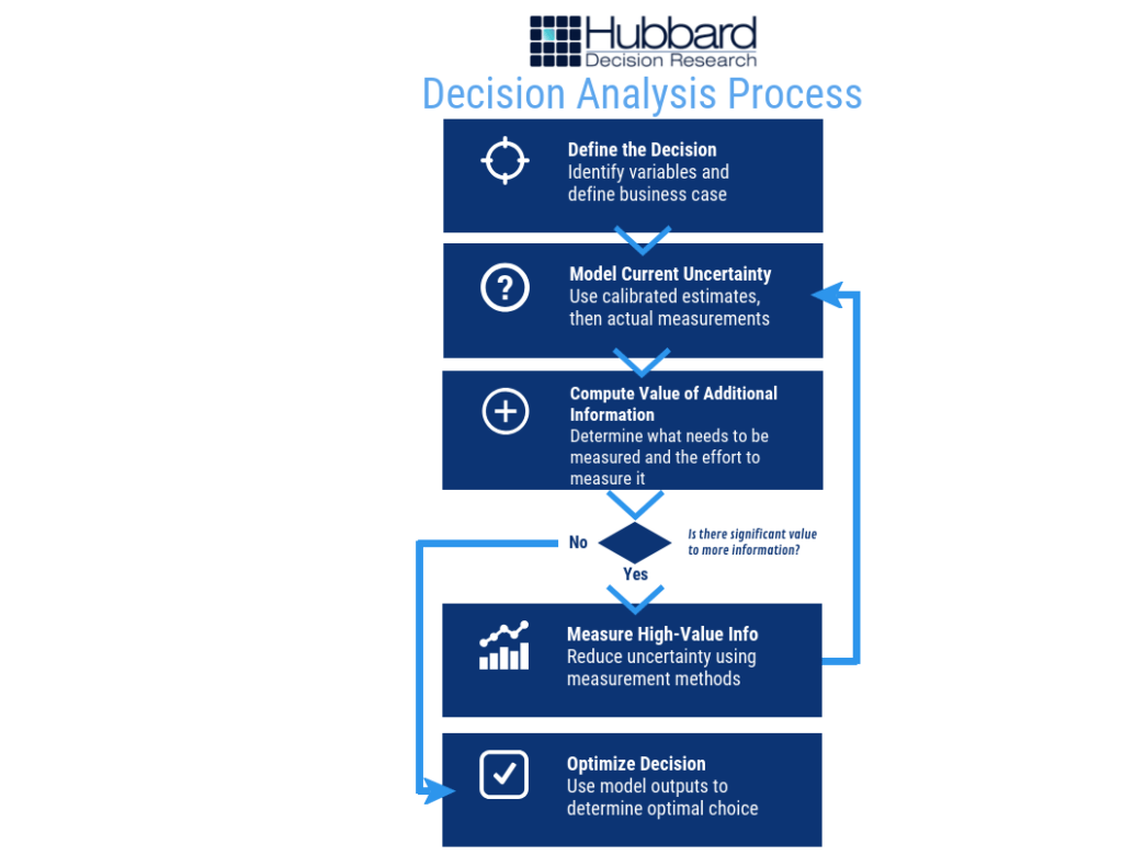
Improved estimation quality forms a critical component of the Applied Information Economics (AIE) framework. Organizations frequently face data gaps. A common reaction treats further analysis as impossible until those gaps are filled, prompting immediate, large-scale data collection. In contrast, AIE emphasizes decision definition and measurement of current knowledge before engaging in such efforts. As illustrated in Figure 2, the framework uses quantitative analysis to show where reducing uncertainty would meaningfully affect the decision.

Figure 2


AIE helps organizations avoid a common decision-making pitfall: Measurement Inversion. As termed by Doug Hubbard, the Measurement Inversion describes a repeatedly observed pattern in which organizations measure and collect data on factors that have little or no effect on decisions. Millions of dollars can be poured into these efforts. Doug Hubbard often remarks, “I honestly wonder how this doesn’t impact the GDP.”  A reasonable response is that it probably does.

The first step of AIE, defining the decision, focuses on the choices under consideration, the outcomes that matter, and the uncertain variables that influence those outcomes. Risk analysis supports better decisions about which risk-reduction actions best serve the organization. Every organization faces many possible mitigations, controls, and initiatives, but determining which are justified requires quantitative analysis. Clear decision definition provides the foundation for prioritization.

Identification of variables that merit additional measurement follows from the next two AIE steps: modeling current knowledge and computing the value of additional information. Modeling current knowledge involves populating the model with “arm’s-reach” data and calibrated estimates. Calibration training ensures that uncertainty around each estimate is represented appropriately. Once the model is populated, analysis proceeds to calculation of the value of information (VOI), which indicates where additional measurement is worth the effort.

For example, consider a hypothetical capital project planning a major facility upgrade. Early cost and schedule data are incomplete, and the team considers delaying approval to collect detailed estimates across all work packages. AIE modeling using calibrated estimates shows that uncertainty in a small number of long-lead components drives most of the risk, while uncertainty in routine tasks has little impact on the decision. VOI analysis confirms that broad data collection would not change the outcome, whereas targeted measurement would.

VOI quantifies the economic impact of reducing uncertainty in specific model inputs. Ron Howard, a founder of decision analysis, introduced the concept in the 1960s, yet organizations still apply it infrequently. Many variables exhibit negligible information value, indicating that additional data collection or analysis would not affect decisions.

Before taking on a large data-collection effort, pause and ask whether that effort is actually justified. Avoid falling prey to Measurement Inversion. In many cases, decisions improve more from well-calibrated estimates than from indiscriminate data gathering. AIE provides a structured way to use calibrated judgment and value-of-information analysis to focus measurement on uncertainty that truly matters and to support better decisions.

What the Manhattan Project and James Bond Have in Common – and Why Every Analyst Needs to Know It

monte carlo simulation

Overview:

  • A powerful quantitative analysis method was created as a result of the Manhattan Project and named for an exotic casino popularized by the James Bond series
  • The tool is the most practical and efficient way of simulating thousands of scenarios and calculating the most likely outcomes
  • Unlike other methods, this tool incorporates randomness that is found in real-world decisions
  • Using this method doesn’t require sophisticated software or advanced training; any organization can learn how to use it

A nuclear physicist, a dashing British spy, and a quantitative analyst walk into a casino. This sounds like the opening of a bad joke, except what all of these people have in common can be used to create better decisions in any field by leveraging the power of probability.

The link in question – that common thread – gets its name from an exotic locale on the Mediterranean, or, specifically, a casino. James Bond visited a venue inspired by it in Casino Royale, a book written by Ian Fleming, who – before he was a best-selling author – served in the British Naval Intelligence Division in World War II. While Fleming was crafting creative plans to steal intel from Nazi Germany, a group of nuclear physicists on the other side of the Atlantic were crafting plans of their own: to unleash the awesome destructive power of nuclear fission and create a war-ending bomb.

Trying to predict the most likely outcome during a theoretical nuclear fission reaction was difficult to say the least, particularly using analog computers. To over-simplify the challenge, scientists had to be able to calculate whether or not the bomb they were building would explode – a calculation that required an integral equation to somehow predict the behavior of atoms in a chain reaction. Mathematicians Stanislaw Ulam and John Von Nuemann, both members of the Manhattan Project, created a way to calculate and model the sum of thousands of variables (achieved by literally placing a small army of smart women in a room and having them run countless calculations). When they wanted to put a name to this method, Ulam recommended the name of the casino where his uncle routinely gambled away large sums of money<fn>Metropolis, N. (1987). The Beginning of the Monte Carlo Method. Los Alamos Science, 125-130. Retrieved from https://permalink.lanl.gov/object/tr?what=info:lanl-repo/lareport/LA-UR-88-9067</fn>.

That casino – the one Fleming’s James Bond would popularize and the one where Ulam’s uncle’s gambling addiction took hold – was in Monte Carlo, and thus the Monte Carlo simulation was born.

Now, the Monte Carlo simulation is one of the most powerful tools a quantitative analyst can use when incorporating the power of probabilistic thinking into decision models.

How a Monte Carlo Simulation Works – and Why We Need It To

In making decisions – from how to make a fission bomb to figuring out a wager in a table game in a casino – uncertainty abounds. Uncertainty abounds because, put simply, a lot of different things can happen. There can be almost-countless scenarios for each decision, and the more variables and measurements are involved, the more complicated the calculations become to try and figure out what’s most likely to happen.

If you can reduce possible outcomes to a range of probabilities, you can make better decisions in theory. The problem is, doing so is very difficult without the right tools. The Monte Carlo simulation was designed to address that problem and provide a way to calculate the probability of thousands of potential outcomes through sheer brute force.

Doug Hubbard provides a scenario in The Failure of Risk Management that explains how a Monte Carlo simulation works and can be applied to a business case (in this context, figuring out the ROI of a new piece of equipment). Assume that you’re a manager considering the potential value of a new widget-making machine. You perform a basic cost-benefit analysis and estimate that the new machine will make one million widgets, delivering $2 of profit per unit. The machine can make up to 1.25 million, but you’re being conservative and think it’ll operate at 80% capacity on average. We don’t know the exact amount of demand. We could be off by as much as 750,000 widgets per year, above or below.

We can conceptualize the uncertainty we have like so:

  • Demand: 250,000 to 1.75 million widgets per year
  • Profit per widget: $1.50 to $2.50

We’ll say these numbers fall into a 90% confidence interval with a normal distribution. There are a lot of possible outcomes, to put it mildly (and this is a pretty simple business case). Which are the most likely? In the book, Doug used an MC simulation to run 10,000 simulations – or 10,000 scenarios – and tallied the results for each (with each scenario representing some combination of demand and profit per widget to create a loss or gain). The results are described by two figures: a histogram of outcomes (figure 1) and a cumulative probability chart (figure 2)<fn>Hubbard, D. W. (2009). The failure of risk management: Why its broken and how to fix it. Hoboken, NJ: J. Wiley & Sons.</fn>:

Figure 1: Histogram of Outcomes

Figure 2: Cumulative Probability Chart

You, the manager, would ideally then calculate your risk tolerance and use this data to create a loss exceedance curve, but that’s another story for another day. As Doug explains, using the MC simulation allowed you to gain critical insight that otherwise would’ve been difficult to impossible to obtain:

Without this simulation, it would have been very difficult for anyone other than mathematical savants to assess the risk in probabilistic terms. Imagine how difficult it would be in a more realistically complex situation.

The best way to sum up the diverse benefits of incorporating MC simulations into decision models was written by a group of researchers in an article titled “Why the Monte Carlo method is so important today”:<fn>Kroese DPBrereton TTaimre TBotev ZIWhy the Monte Carlo method is so important todayWiley Interdisciplinary Reviews: Computational Statistics 201466): 386– 392.</fn>

  • Easy and Efficient. Monte Carlo algorithms tend to be simple, flexible, and scalable.
  • Randomness as a Strength. The inherent randomness of the MCM is not only essential for the simulation of real-life random systems, it is also of great benefit for deterministic numerical computation.
  • Insight into Randomness. The MCM has great didactic value as a vehicle for exploring and understanding the behavior of random systems and data. Indeed we feel that an essential ingredient for properly understanding probability and statistics is to actually carry out random experiments on a computer and observe the outcomes of these experiments — that is, to use Monte Carlo simulation.
  • Theoretical Justification. There is a vast (and rapidly growing) body of mathematical and statistical knowledge underpinning Monte Carlo techniques, allowing, for example, precise statements on the accuracy of a given Monte Carlo estimator (for example, square-root convergence) or the efficiency of Monte Carlo algorithms.

Summarized, Monte Carlo simulations are easy to use, not only help you more closely replicate real-life randomness but understand randomness itself, and are backed by scientific research and evidence as to how they make decision models more accurate. We need them to work because any significant real-world decision comes with a staggering amount of uncertainty, complicated by thousands of potential outcomes created by myriad combinations of variables and distributions – all with an eminently-frustrating amount of randomness haphazardly mixed throughout.

How to Best Use a Monte Carlo Simulation

Of course, knowing that an MC simulation tool is important – even necessary – is one thing. Putting it into practice is another.

The bad news is that merely using the tool doesn’t insulate you from a veritable rogue’s gallery of factors that lead to bad decisions, ranging from overconfidence to using uncalibrated subjective estimates, falling victim to logical fallacies, and making use of soft-scoring methods, risk matrices, and other pseudo-quantitative methods that aren’t better than chance and frequently worse.

The good news is that all of those barriers to better decisions can be overcome. Another piece of good news: you don’t need sophisticated software to run a Monte Carlo simulation. You don’t even need specialized training. Many of the clients we train in our quantitative methodology don’t have either. You can actually build a functional MC simulation in native Microsoft Excel. Even a basic version can help by giving you more insight than you know now; by giving you another proven way to glean actionable knowledge from your data.

On its own, though, a MC simulation isn’t enough. The best use of the Monte Carlo method is to incorporate it into a decision model. The best decision models employ proven quantitative methods – including but not limited to Monte Carlo simulations – to follow the process below (figure 3):

decision analysis process

Figure 3: HDR Decision Analysis Process

The outputs of a Monte Carlo simulation are typically shown in that last step, when the model’s outputs can be used to “determine optimal choice,” or, figure out the best thing to do. And again, you don’t need specialized software to produce a working decision model; Microsoft Excel is all you need.

You may not be creating a fearsome weapon, or out-scheming villains at the baccarat table, but your decisions are important enough to make using the best scientific methods available. Incorporate simulations into your model and you’ll make better decisions than you did before – decisions a nuclear physicist or a secret agent would admire.


Recommended Products:

Learn how to create Monte Carlo simulations in Excel with our Basic Simulations in Excel webinar. Register today to get 15% off with coupon code EXCEL15.