by Joey Beachum | Mar 27, 2019 | Announcements, Articles, General Topics, News
 Science, we have a problem. Several problems, actually. Now we have solutions. A central tenant of modern science is that experiments must be reproducible. It turns out that a surprisingly large proportion of published results in certain fields of research – especially in the social and health sciences – do not satisfy that requirement. This is known as the reproducibility crisis.
I was honored to have the opportunity to be involved in addressing this as both an associate editor of a ground-breaking special Issue of The American Statistician and to co-author one of the 43 articles. This special issue is called “Moving to a World Beyond p<.05” Some of my readers will recognize that “p<.05” refers to the “significance test”, ubiquitous in scientific research. This issue is the first serious attempt to fundamentally rethink statistical inference in science since the significance tests currently used were developed almost a century ago.
The article I authored with Alicia Carriquiry (Distinguished Professor of Statistics at Iowa State University) is titled Quality Control for Scientific Research: Addressing Reproducibility, Responsiveness, and Relevance. We argue that addressing responsiveness and relevance will help address reproducibility. Responsiveness refers to the fact it takes a long time before problems like this are detected and announced. The discovery of the current problems of reproducibility only occurred because, periodically, some diligent researchers decided to investigate it. Years of unreproducible studies continue to be published before these issues are known and even longer before they are acted on.
Relevance refers to how published research actually supports decisions. If the research is meant to inform corporate or public decisions (it is certainly often used that way) then it should be able to tell us the probability that the findings are true. Assigning probabilities to potential outcomes of decisions is a vital step in decision theory. Many who have been using scientific research to make major decisions would be surprised to learn that the “Null Hypothesis Significance Test” (NHST) does not actually tell us that.
However, Alicia and I show a proof about how this probability could be computed. We were able to show that we can compute the relevant probability (i.e., that the claim is true) and that even after a “statistically significant” result the probability is, in some fields of research, still less than 50%. In other words, a “significant” result doesn’t mean “proven” or even necessarily “likely.” A better interpretation would be “plausible” or perhaps “worth further research.” Only after the results are reproduced does the probability the hypothesis is true start to grow to about 90%. This would be disappointing for policy makers or news media that tend to get excited about the first report of statistical significance. In fact, measuring such probabilities can be the basis of a sort of quality control for science that can be much more responsive as well as relevant. Any statistically significant result should be treated as a tentative finding awaiting further confirmation.
Now, a little background to explain what is behind such an apparently surprising mathematical proof. Technically, a “statistically significant” result only means that if there were no real phenomena being observed (the “null” hypothesis) then the statistical test result – or something more extreme – would be unlikely. Unlikely in this context means less than the stated significance level, which in many of the research fields in question is 0.05. Suppose you are testing a new drug that, in reality, is no better than a placebo. If you would have run an experiment 100 times you would, by chance alone, get a statistically significant result in about 5 experiments at a significance level of .05. This might sound like a tested hypothesis with a statistically significant result has a 95% chance of being of being true. It doesn’t work that way. First off, if you only publish 1 out of 10 of your tests, and you only publish significant results, then half of your published results are explainable as chance. This is called “publication bias.” And if a researcher has a tendency to form outrageous hypotheses that are nearly impossible to be true, then virtually all of the significant results would be the few random flukes we would expect by chance. If we could actually compute the probability the claim is true, then we would have a more meaningful and relevant test of a hypothesis.
One problem with answering relevance is that it requires a prior probability. In other words, we have to have to be able to determine a probability the hypothesis is true before the research (experiment, survey, etc.) and then update it based on the data. This reintroduces the age-old debate in statistics about where such priors come from. It is sometimes assumed that such priors can only be subjective statements of an individual, which undermines the alleged objectively of science (I say alleged because there are several arbitrary and subjective components of statistical significance tests). We were able to show that an objective prior can be estimated based on rate at which studies in a given field can be successfully reproduced.
In 2015, a group called The Open Science Collaboration tried to reproduce 100 published results in psychology. The group was able to reproduce only 36 out of 100 of the published results. Let’s show how this information is used to compute a prior probability as well as the probability the claim is true after the first significant results and after it is reproduced.
The proposed hypothesis the researcher wants to test the truth of is called “alternative” to distinguish it from the null hypothesis, where the results were a random fluke. The probability that the alternative hypothesis is true, written Pr(Ha), based only on the reproducibility history of a field, is:

Where R is the reproducibility rate, and α and π refer to what is known as the “significance level” and the statistical “power” of the test. I won’t explain those in much detail but these would be known quantities for any experiment published in the field.
Using the findings of The Open Science Collaboration, R would be .36 (actually we would use those results as a sample to estimate the reproduction rate which itself would have an error, but we will gloss over that here). The typical value for α is .05 and π is, on average, perhaps as high as .8. This means that that hypothesis being considered for publication in that field have about a 4.1% chance of being true. Of course, you would expect that researchers proposing a hypothesis probably have reason to believe they have some chance that what they are testing is true but before the actual measurement, the probability isn’t very high. After the test is performed, the following formula shows the probability is a claim is true given that it passed the significance test (shown as the condition P< α).

What might surprise many decision makers who might want to act on these findings that that, in this field of research, a “significant” result using an experiment with the same α and π means that now we can say that the hypothesis has only a 41.3% chance of being true. When (and if) the result is ever successfully reproduced it, the probability the hypothesis is true is adjusted again to 91.9% with the following formula.

If we plot all three of these probabilities as a function of reproduction rate for a given α and π, we get a chart like the following.
Probability the hypothesis is true upon initial proposal, after the first significant result and after reproduction
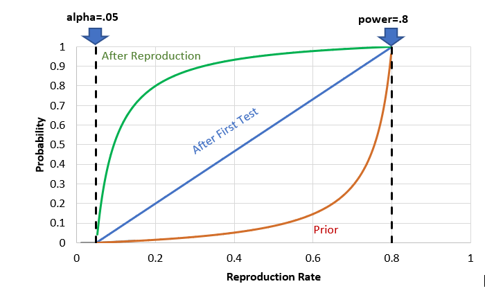
Other reproduction attempts similar to The Open Science Collaboration show replication rates well short of 60% and more often below 50%. As the chart shows, if we wanted to have a probability of at least 90% that a hypothesis is true before making a policy decision, reproduction rates would have to be on the order of 75% or higher holding other conditions constant. In addition to psychology, these findings affect issues as broad as education policy, public health, product safety, economics, sociology, and many other fields where significance tests are normal practice.
Alicia and I proposed that Pr(Ha) itself becomes an important quality control for fields of research like psychology. Instead of observing problems perhaps once every decade or two, Pr(Ha) can be updated with each new reproduction attempt and that will update all of the Pr(Ha|P<a) in the field at a rate closer to real time. Now, our paper is only one of 43 articles in this massive special issue. There are many articles that will be very important in rethinking how statistical inference has been applied for many decades.
The message across all the articles is the same – the time for rethinking quality control in science is long overdue and we know how to fix it.
– Doug Hubbard
by Joey Beachum | Dec 26, 2018 | News, Uncategorized

During the course of a typical day, humans will make an enormous amount of conscious and subconscious decisions. Not all of those decisions are what we’d call crucial. The vast majority aren’t. But every day, we’ll make several decisions that matter – that have a significant impact on how our lives unfold.
When we’re trying to decide on a course of action from the multitude of options we typically have, we’re trying to, at the very least, predict the future. (Not in an psychic sense, of course.) In other words, we’re assessing the options we have and calculating the probability that decision A will result in outcome A, B, or C – while also figuring out how good or bad outcomes A, B, or C would be if they happened.
Of course, we all want to make good decisions. But we don’t always do that – and sometimes, our bad decisions are catastrophic.
As we’re about to cover, there are several reasons why humans make poor decisions, ranging from cognitive biases to simply not using the right processes. We’ll also cover what you can do to put yourself in a position to make better calls and do a better job of predicting outcomes and assessing probabilities.
The takeaway will be simple: If you do the right things, your decision-making ability will measurably improve – and a good number of those bad decisions can be changed for the better.
A Decision-Maker’s Most Formidable Foe: Uncertainty
Think about some of the decisions you’ve had to make in your life.
If you went to college, you had to pick one. If you’re married, or engaged, you had to find a partner and decide to propose – or accept a proposal. In your job, maybe you had to decide what investment to make, or what actions to take. If you’re a business owner, you had to make a ton of important decisions that led to where you are today, for better or for worse.
In every single one of those decisions, you didn’t know for sure what would happen. Even if you thought it was a 100% sure thing, it probably wasn’t, because there are few sure things in the world. When there is more than one possible outcome, and you’re not sure which one will occur, you experience something called uncertainty, and it can be quantified on a 0-100% scale (such as being 90% sure your partner is going to say yes to your proposal, or only 50% sure – the same as a coin flip – that your big investment is going to pay off.)
Usually, hard decisions – the decisions that determine success versus failure – involve dozens of variables that lead to multiple possible outcomes. With each variable and potential outcome comes a great deal of uncertainty – so much at times, in fact, that it’s a wonder decisions are made at all.
In short, we deal with uncertainty every single day, with every decision we make. The tougher the decision, the more uncertainty – or, should we say, the more uncertainty, the tougher the decision.
Being better at assessing probabilities, making decisions, and predicting the future is all about reducing uncertainty as much as possible. If you can reduce the amount of uncertainty you face, whether you’re figuring out how likely something is to happen or trying to predict what will happen in the future, you’ll be more likely to make the right call.
The trouble is, humans are bad at assessing probabilities and predicting the future. Research has shown why this is the case. Daniel Kahneman, with Amos Tversky, won a Nobel Prize in Economics for showing how humans are subject to a wide array cognitive biases based on how much we rely on erroneous judgmental heuristics.
Researchers Baruch Fischhoff, Paul Slovic, and Sarah Lichtenstein found that humans are psychologically biased toward unwarranted certainty, i.e. we tend to be overconfident when we make judgments due to a variety of reasons, such as our memories being incomplete and erroneously recalled. Put another way, we are often extremely overconfident when we think we’re right about something, especially when we rely on our experience (or rather, our perceptions of that experience).
Psychologist and human judgment expert Robyn Dawes confirmed the effect of these limitations when he found that expert judgment is routinely outperformed by actuarial science (i.e. hard quantitative analysis) when it came to making decisions.
Social psychologists Richard Nisbett and Lee Ross explained how “Stockbrokers predicting the growth of corporations, admissions officers predicting the performance of college students, and personnel managers choosing employees are nearly always outperformed by actuarial formulas.”
Put together, there are many reasons why we, as a species, are not terribly good at figuring out what is going to happen and how likely it is to happen. When you’re trying to make decisions in a world of uncertainty – i.e. every time you try to make a decision – you’re fighting against your brain.
Does that mean we should just concede to our innate biases, misconceptions, and flaws? Does it mean that there’s no real way to improve our ability to reduce uncertainty, mitigate risk, and make better decisions?
Fortunately for us, there are ways to get better at assessing how likely something is to happen, reducing uncertainty, and giving yourself a better chance at making the right call.
Calibration: Making Yourself a Probability Machine
In May, 2018, the United States Supreme Court struck down a federal ban on sports betting. Before that decision, only four states allowed sports betting in any capacity. Since the decision, most states have either legalized sports betting, passed a bill to do so, or introduced a bill to make betting legal within their boundaries.
When we bet on sports, we’re essentially predicting the future (or as Doug says, trying to be less wrong). We’re saying, “I will wager that the New England Patriots will beat the New York Jets,” or that “The Houston Rockets will lose to the Golden State Warriors but only by less than five points.”
When we place a bet, we’re gambling that our confidence in the outcome we’re predicting is better than 50/50, which is a coin flip. Otherwise, there’s no point in making a bet. So, in our heads, we think, “Well, I’m pretty sure New England is the better team.” If we’re the quantitative type, we try to put a percentage to it: “I’m 70% confident that the Rockets can keep it close.”
Putting a percentage on uncertainty is good; the first step when reducing uncertainty is to quantify it. But simply slapping an arbitrary number on your confidence creates problems, namely, how accurate is your number?
In other words, if you’re 70% confident, the event should happen 70% of the time. If it happens more frequently, you were underconfident; if it happens less frequently (as is usually the case), then you were overconfident and could potentially lose a lot of money.
The range of probable values that you create to quantify your uncertainty is called a confidence interval (CI). If you’re betting on sports – or anything, really – then you can quantify uncertain by giving yourself a certain range of possibilities that you think are likely depending on your confidence.
For example, let’s say that Golden State is predicted by Vegas bookies to beat Houston by 5 or more points. You think, “Well, there’s no way they lose, so the minimum amount they’ll win by is one point, and they could really blow Houston out, so let’s say the most they’ll win by is 12 points.” That’s your range. Let’s say you think you’re 90% confident that the final margin of victory will be within that range. Then, you are said to have a 90% CI of one to 12.
You’ve now quantified your uncertainty. But, how do you know your numbers or your 90% CI are good? In other words, how good are you at assessing your own confidence in your predictions?
One way to figure out if someone is good at subjective probability assessments is to compare expected outcomes to actual outcomes. If you predict that particular outcomes will happen 90% of the time, but they only happened 80% of the time, then perhaps you were overconfident. Or, if you predict that outcomes will happen 60% of the time, but they really happened 80% of the time, you were underconfident.
This is called being uncalibrated. So, it follows that being more accurate in your assessments is being calibrated.
Calibration basically is a process by which you remove estimating biases that interfere with assessing odds. This process has been a part of decision psychology since the 1970’s, yet it’s still relatively unknown in the broader business world. A calibrated person can say that an event will happen 90% of the time, and 90% of the time, it’ll happen. They can predict the outcome of 10 football games with a 90% CI and hit on 90% of them. If they say they’re 90% sure that the Patriots will beat the Jets, they can make a bet and 90% of the time, they’ll be right.
More broadly speaking, a calibrated person is neither overconfident or underconfident when assessing probabilities. This doesn’t mean the person is always right; they won’t be. (Doug Hubbard talks about how a 90% CI is more useful than a 100% CI, or saying the outcomes outside of your range absolutely won’t happen, which isn’t often the case in the real world). It just means that they are better at estimating probabilities than other people.
Put very simply, as Doug does in his book, How to Measure Anything, “A well calibrated person is right just as often as they expect to be – no more, no less. They are right 90% of the time they say they are 90% confident and 75% of the time they say they are 75% confident.”
The unfortunate news is that the vast majority of people are uncalibrated. Very few people are naturally good at probabilities or predicting the future.
The fortunate news is that calibration can be taught. People can move from uncalibrated to calibrated through special training, such as our calibration training, and it’s easier than you think.
Consider the image below (Figure 1). This is a list of questions and statements from our calibration training sessions we offer. The top half contains a list of 10 trivia questions. We ask participants to give us a 90% CI – i.e. a range of values in which they’re 90% sure the correct answer will be. So, for the first question, a participant may be 90% certain that the actual answer is anywhere from 20 mph to 400 mph.
For the second list, we ask participants to answer true or false and mark their confidence that they are correct.
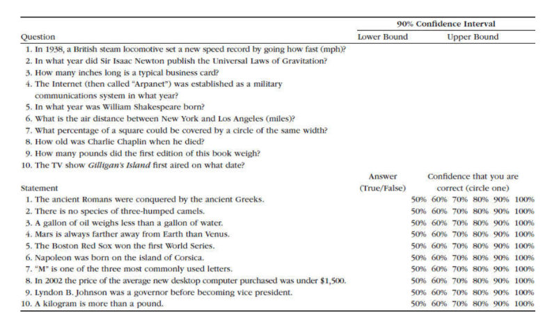
Figure 1: Sample of Calibration Test
Some of those questions may be very difficult to answer. Some might be easy. Whether you know the right answer or not isn’t the point; it’s all about gauging your ability to assess your confidence and quantify your uncertainty.
After everyone is finished, we share the actual answers. Participants get to see how well their assessments of their confidence stack up. We then give feedback and repeat this process across a series of tests that we’ve designed.
What most people find is that they are very uncalibrated, and usually quite overconfident. (Remember from earlier the research that shows how people tend to be naturally overconfident in their assessments and predictions). We also find people that are underconfident.
Over the course of the training session, however, roughly 85% of participants will become calibrated, in that they’ll hit on 90% of the questions. That’s because during the training, we share with them several proven techniques that they can use throughout the testing to help them make better estimates.
A combination of technique and practice, with feedback, results in calibration. As you can see in the image below (Figure 2), calibrated groups outperform uncalibrated groups when evaluating their confidence in predicting outcomes.
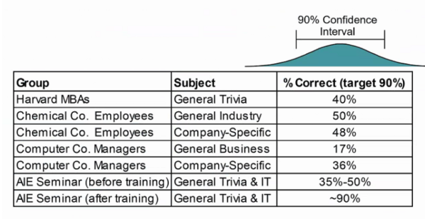 Figure 2: Comparison of Uncalibrated versus Calibrated Groups
Long story short, calibration is a necessary part of making subjective assessments of probabilities. You can’t avoid the human factor in decision-making. But you can reduce uncertainty and your chance of error by getting better at probabilities by becoming calibrated, which means your inputs to a decision-making model will be more useful.
Quantitative Tools to Help Make Better Decisions
Calibration alone won’t turn you into a decision-making prodigy. To go even further, you need numbers – but not just any numbers and not just any method to create them.
The use of statistical probability models in decision-making today is a relatively new thing. The field of judgment and decision-making (JDM) didn’t emerge until the 1950’s, and really took off in the 1970’s and 1980’s through the work of Nobel laureate Daniel Kahneman (most recently the author of bestseller Thinking Fast and Slow) and his collaborator, Amos Tversky.
JDM is heavily based on statistics, probability, and quantitative analysis of risks and opportunities. The idea is that a well-designed quantitative model can remove many of the cognitive biases that are innate to mankind that interfere with making good decisions. As mentioned previously, research has borne that out.
One striking example of how statistics evolved in the 20th Century to allow analysts to make better inferences came during World War II, as told by Doug in How to Measure Anything. The Allies were very interested in how many Mark V Panther tanks Nazi Germany could produce, since armor was arguably Germany’s most dominant weapon (alongside the U-boat) and the Mark V was a fearsome weapon. They needed to know what kind of numbers they’d face in the field so they could prepare and plan.
At first, the Allies had to depend on spy reports. These are very inconsistent. Allied intelligence cobbled together these reports and came up with estimates of monthly production ranging from 1,000 in June 1940 to 1,550 in August 1942.
In 1943, however, statisticians took a different approach. They used a technique called serial sampling to sample tank production using the serial numbers on captured tanks. As Doug says, “Common sense tells us that the minimum tank production must be at least the difference between the highest and lowest serial numbers of captured tanks for a given month. But can we infer even more?”
The answer was yes. Statisticians treated the captured tank sample as a random sample of the entire tank population and used this to compute the odds of different levels of production.
Using these statistical methods, these analysts were able to come up with dramatically different – and far more accurate – tank production estimates than what Allied intelligence could produce from its earlier reports (see Figure 3).
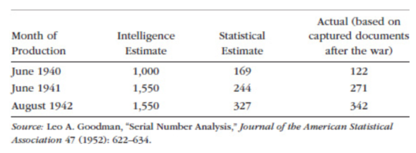
Figure 3: Results of the Serial Number Analysis
The military would go on to become a believer in quantitative analysis, which would spread to other areas of government and also the private sector, fueled by the emergence of computers that could handle increasingly-sophisticated quantitative models.
A Sampling of Quantitative Tools and Models
Today, a well-designed quantitative model takes advantage of several key tools and methods that collectively do a better job of analyzing all of the variables and potential outcomes in a decision and informing the decision-maker with actionable insight.
These tools include:
- Monte Carlo simulations: Developed during World War II by scientists who were working on the Manhattan Project, Monte Carlo simulations analyzes risks through modeling all possible results via repeated simulations using a probability distribution. Thousands of samples are generated to create a range of possible outcomes to give you a comprehensive picture of not just what may occur, but how likely it is to occur.
- Bayesian analysis: Named for English mathematician Thomas Bayes, Bayesian analysis combines prior information for a parameter (or variable) with a sample to produce a range of probabilities for that parameter. It can be easily updated with new information to produce more relevant probabilities.
- Lens Method: Developed by Egon Brunswick in the 1950’s, this method measures and removes significant sources of errors in expert judgments due to estimator inconsistency through a regression model.
- Applied Information Economics (AIE): AIE combines several methods from economics, actuarial science, and other mathematical disciplines to define the decision at hand, measure the most important variables and factors, calculate the value of additional information, and create a quantitative decision model to inform the decision-maker.
The result of all methods put together is a model, which can take data inputs and produce a statistical output that helps a decision-maker make better decisions.
Of course, the outputs are only as good as the inputs and the model itself, and not all inputs are important. The model, first, has to be based on sound mathematical and scientific principles. Second, the inputs have to be useful – but most of them aren’t. This is a concept Doug Hubbard calls measurement inversion (see Figure 4).
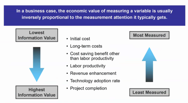
Figure 4: Measurement Inversion
Put simply, decision-makers and analysts think certain variables are important and should be measured, and ignore other variables that are deemed as unimportant or immeasurable. Ironically, the variables they think are relevant usually aren’t, and the ones they think aren’t relevant are usually the things they most need to measure.
In Figure 5, you can see real-world examples of measurement inversion, as uncovered through the past 30 years of research Hubbard Decision Research has conducted.
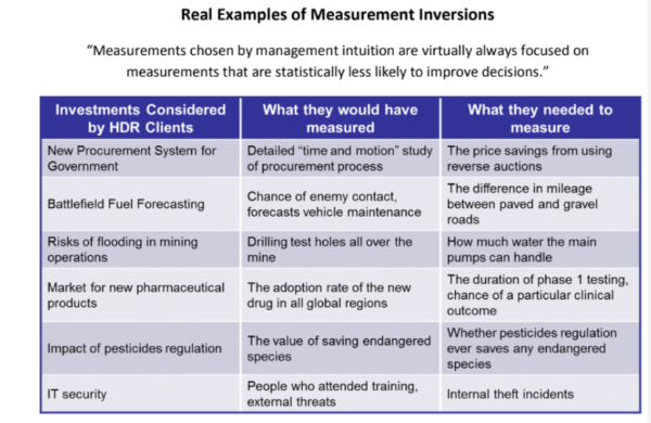
Figure 5: Real-World Examples of Measurement Inversion
These and other cases of measurement inversion have been backed by research and statistical analysis. What’s often the case is that a decision-maker is basing decisions on outputs from a model that is either not sound, or – more dangerously – is sound yet is getting fed erroneous or irrelevant data.
One thing AIE does is calculate the value of information. What’s it worth to us to take the effort to measure a particular variable? If you know the value of the information you have and can gather, then you can measure only what matters, and thus feed your model with better inputs.
With the right inputs, and the right model, decision-makers can make decisions that are measurably better than what they were doing before.
Conclusion: Making Better Decisions
If a person wants to become better at making decisions, they have to:
- Recognize their innate cognitive biases;
- Calibrate themselves so they can get better at judging probabilities; and
- Use a quantitative method which has been shown in published scientific studies to improve estimates or decisions.
The average person doesn’t have access to a quantitative model, of course, but in the absence of one, the first two will suffice. For self-calibration, you have to look back at previous judgments and decisions you’ve made and ask yourself hard questions: Was I right? Was I wrong? How badly was I wrong? What caused me to be so off in my judgment? What information did I not take into consideration?
Introspection is the first step toward calibration and, indeed, making better decisions in general. Adopting a curious mindset is what any good scientist does, and when you’re evaluating yourself and trying to make better decisions, you’re essentially acting as your own scientist, your own analyst.
If you’re a decision-maker who does or can have access to quantitative modeling, then there’s no reason to not use it. Quantitative decision analysis is one of the best ways to make judgment calls based on empirical evidence, instead of mere intuition.
The results speak for themselves: decision-makers who make use of the three steps outlined above really do make better decisions – and you can actually measure how much better they are.
You’ll never be able to gaze into a crystal ball and predict the future with 100% accuracy. But, you’ll be better at it than you were before, and that can make all the difference.

by Joey Beachum | Nov 6, 2018 | How To Measure Anything Blogs, News
When it comes to statistics, there are a lot of misconceptions floating around. Even people who have scientific backgrounds subscribe to some of these common misconceptions. One misconception that affects measurement in virtually every field is the perceived need for a large sample size before you can get useful information from a measurement.
Measurements are often dismissed, without doing any actual math, because someone believes they need a larger sample size to be “statistically significant.” We see examples of this line of thought everywhere. In sports, for example, we dismiss predictive metrics because they naturally work with small sample sizes (a season is only so long, with only so many games, after all), choosing instead to go with “gut feel” and “expert knowledge.”
In other words, a measurement isn’t useless if the sample size is small. You can actually use small sample sizes to learn something useful about anything – even, as we’ll soon see, with really small samples.
And if you can learn something useful using the limited data you have, you’re one step closer to measuring anything you need to measure – and thus making better decisions. In fact, it is in those very situations where you have a lot of uncertainty, that a few samples can reduce uncertainty the most. In other words, if you know almost nothing, almost anything will tell you something.
In How to Measure Anything: Finding the Value of Intangibles in Business, Doug Hubbard uses two under-the-radar statistical principles to demonstrate how even small amounts of data can provide a lot of useful insight: the Rule of Five and the Urn of Mystery.
The Rule of Five
Pretend for a moment that you’re a decision-maker for a large corporation with 10,000 employees. You’re considering automating part of some routine activity, like scheduling meetings or preparing status reports. But you are facing a lot of uncertainty and you believe you need to gather more data. Specifically, one thing you’re looking for is how much time the typical employee spends each day commuting.
How would you gather this data?
You could create what essentially would be a census where you survey each of the 10,000 employees. But that would be very labor-intensive and costly. You probably wouldn’t want to go through that kind of trouble. Another option is to get a sample, but you are unsure what the sample size should be to be useful.
What if you were told that you might get enough information to make a decision by sampling just five people?
Let’s say that you randomly pick five people from your company. Of course, it’s hard for humans to be completely random, but let’s assume the picking process was about as random as you can get.
Then, let’s say you ask these five people to give you the total time, in minutes, that they spend each day in this activity. The results come in: 30, 60, 45, 80, and 60 minutes. From this, we can calculate the median of the sample results, or the point at which exactly half of the total population (10,000 employees) is above the median and half is below the median.
Is that enough information?
Many people, when faced with this scenario, would say the sample is too small – that it’s not “statistically significant.” But a lot of people don’t know what statistically significant actually means.
Let’s go back to the scenario. What are the chances that the median time spent in this activity for 10,000 employees, is between 30 minutes and 80 minutes, the low and high ends, respectively, of the five-employee survey?
When asked, people often say somewhere around 50%. Some people even go as low as 10%. It makes sense, after all; there are 10,000 employees and countless individual commute times in a single year. How can a sample that is viewed as not being statistically significant possibly get close?
Well, here’s the answer: the chances that the median time spent of the population of 10,000 employees is between 30 minutes and 80 minutes is a staggering 93.75%.
In other words, you can be very confident that the median time spent is between 30 minutes and 80 minutes, just by asking five people out of 10,000 (or 100,000, or 1,000,000 – it’s all the same math).
This may seem like a wide range, but that’s not the point. The relevant point is whether this range is narrower than your previous range. Maybe you previously thought that 5 minutes per day or 2.5 hours per day were reasonable given what you knew at the time. These values now would be highly unlikely to be medians for the population. Even with a small measurement of just five people, you significantly narrowed your range of uncertainty. If your uncertainty was that high before, you now have a much better idea.
Now suppose the proposed investment breaks even if the median time spent is 10 minutes per person per day. That is, if the median time spent is any higher than 10 minutes, the proposed investment will do better than break even. In this case you’ve already reduced uncertainty enough to be confident in a decision to invest. Likewise, you would be confident to reject the investment if the breakeven was 2 hours. If your break even was, say 45 minutes, you might consider further sampling before you make a decision.
So, making better decisions is all about getting valuable information from measuring data. But it doesn’t take a lot of data to give you something useful to work with.
What if you could learn something useful with even less information?
The Urn of Mystery
Picture yourself in a warehouse. In front of you stands a man – we’ll say that he is dressed like a carnival barker, complete with fancy red coat, a top hat, and a mischievous look on his face. (This is a far cry from your usual corporate office environment.)
The carnival barker waves his arm toward the inside of the warehouse. You see rows and rows of large urns. You try to count them but they just keep going and going into the dark recesses of the warehouse.
“Each urn,” he says to you, “is filled with marbles – let’s say 100,000 marbles per urn. Every marble in these urns is either red or green. But, the mixture of red and green marbles varies from urn to urn. An urn could have 100% green marbles and 0% red marbles. Or 33% green marbles and 67% red marbles. Or it could be an even split, 50-50. Or anything else in between 0 to 100%. All percentages are equally likely. And assume that the marbles in each urn have been thoroughly and randomly mixed.”
The barker continues. “Here’s my proposition. We’ll play a betting game. We’ll choose an urn at random. Then, I’ll bet that the marbles in that urn are either mostly red or mostly green. I’ll give you 2-to-1 odds, and each time you’ll bet $10. That is, if I guess correctly, you lose $10. If I’m wrong, you will win $20. We’ll play through 100 urns. Wanna take the bet?” he asks with a smile.
You know that if it’s a uniform distribution, where all percentages are equally likely, the barker will be right 50% of the time. That means your average gain per bet is $5 (a 50% chance of losing $10 and 50% of gaining $20=(0.5)(-10)+(0.5)(20)=5). So, over 100 urns, you’ll net about $500 – give or take $100 or so – by the end of the game. Sounds like a smart bet.
“It’s a deal,” you say.
“Well, let’s make it a bit more fair for me,” the barker says. “Let me draw just one marble, chosen at random, from an urn before I make my pick. This will be completely random. There’s a special spigot at the bottom that will give me a single marble without allowing me to see the rest. Will you still play the game with me?”
You are probably like most people in thinking that one little marble in a large urn full of marbles isn’t going to matter. It’s too small of a sample size, right?
“You’re on,” you say, and the barker grins because he know he has you.
Most people think that the additional information either doesn’t help the barker at all or provides, at best, a small, marginal advantage – that he’ll win 51% of the time as opposed to 50%, or something like that. After all, there are 100,000 marbles.
If you’re still getting 2-to-1 odds, 51% isn’t much different than 50%. You’ll still win.
Do you know the barker’s new win percentage? Believe it or not, by taking just one sample out of each urn, his win percentage jumps from 50% to 75%. That’s an increase of 50%. So you’ll actually walk away from the game a loser.
This is called the Single Sample Majority Rule, which put formally says, “Given maximum uncertainty about a population proportion – such that you believe the proportion could be anything between 0% and 100% with all values being equally likely – there is a 75% chance that a single randomly selected sample is from the majority of the population.”
You now have actionable insight, more than you had before you started, with one, simple sample. Better walk away from this bet.
Applying These Principles to Measuring Anything
What the Rule of Five and Urn of Mystery teach you is this: when you attempt to measure something, assuming your methods are sound, you’re giving yourself more actionable data for better decisions that is better than simple intuition or gut feel.
Our intuition is often wrong when it comes to statistics and quantitative analysis. We can’t possibly believe that we can gain anything useful from a small sample size. And then there’s the issue of statistical significance.
Here’s the thing: when you measure something, you reduce your uncertainty, which is the best thing you can do to make a better decision. And when you have a lot of uncertainty (e.g., in the case of the urns where the share of marbles of a specific color could be anywhere between 0 and 100%), then even the first random sample can reduce uncertainty a lot.
The first step, though, is to believe that your intuition about statistics, probability, mathematics, and quantitative analysis is probably wrong. There are misconceptions keeping you from making better decisions through measuring and analyzing data. Decision-makers deal with these misconceptions all the time, and the result is that they’re not making the best decisions that they possibly could.
If you can get past raw intuition, or “gut feel,” like so many decision-makers and experts bank on, and you embrace quantitative decision analysis, you can gather more information even using ridiculously small sample sizes like in the Rule of Five or Urn of Mystery.
Don’t be afraid of not knowing what to measure, though. David Moore, former president of the American Statistical Association, once said, “If you don’t know what to measure, measure anyway. You’ll learn what to measure.” Doug calls this the Nike method: the “Just do it” school of thought.
You don’t need a large sample size to begin to measure something, even an intangible that you think is impossible to measure. Even with a small sample size, you can reduce your range of uncertainty – and, therefore, be on your way to making better decisions.
 Science, we have a problem. Several problems, actually. Now we have solutions. A central tenant of modern science is that experiments must be reproducible. It turns out that a surprisingly large proportion of published results in certain fields of research – especially in the social and health sciences – do not satisfy that requirement. This is known as the reproducibility crisis.


 Figure 2: Comparison of Uncalibrated versus Calibrated Groups


 On August 3, 2007, the first edition of How to Measure Anything was published. Since then, Doug Hubbard has written two more editions, three more books, in eight languages for a total of over 100,000 books sold. How to Measure Anything is required reading in several university courses and is now required reading for the Society of Actuaries Exam prep.