Robert Weant, Author at Hubbard Decision Research

Optimizing Prices for Project Bids

by Robert Weant | Mar 7, 2024 | Case Studies

Summary: By measuring how their experts price projects and price elasticity, HDR was able to build our client a pricing model that tripled their operating income.

A few years ago, a medium-sized manufacturing firm came to HDR to help redefine how they quote projects. This firm was in a business environment where their experts would give out unique quotes for custom projects of varying scale and scope. Due to the unique nature of each project, the experts at the firm lacked generalizable data to inform consistent pricing decisions. The firm instead relied on a combination of expert intuition and project cost estimates when quoting prices for a project.

As a senior quantitative analyst at HDR, I was tasked with modeling their existing pricing structure to identify areas for improved consistency and optimization. Using the following high-level steps resulted in margins increasing by 48% and operating income tripling within 18 months of implementing our models.

Model How they Currently Price Project Quotes
Model Price Elasticity
Model Constraints and Optimize Portfolio

Creating a Baseline Using the Lens Method

At HDR we often hear “We simply don’t have enough data.” or” We face too many unique factors.” from clients when describing why they have difficulty quantifying fundamental aspects of their business. Yet there are certain methods we routinely use that can address these perceived limitations, all of which are illusions. One method that addresses these limitations is the Lens Method.

The Lens Method is a regression-based approach that has been used in different industries for decades and has been shown to measurably reduce inconsistency in forecasting models. To develop a lens Model, HDR works with clients to define and identify potential factors that may affect key output metrics. After the factors (or attributes) have been identified, we then generate hundreds of hypothetical scenarios leveraging different combinations of variables for experts to review and estimate the key metric we are trying to measure. In this client’s case, the key metrics we were attempting to measure were the price they would quote to the client and the probability of winning the project. We created 150 hypothetical scenarios that contained factors that our client would consider when quoting a project.

After gathering their responses to these scenarios, we were able to generate a model that would predict how the expert would price a potential project and what probability of winning the project they would assign. What’s more, the model of the experts would outperform the experts themselves. This is due to human judgment being very susceptible to noise. These lens models were used as a basis for our client when pricing potential projects and estimating the probability of winning the project.

Measuring Price Elasticity

The next phase of the work was focused on measuring price elasticity or bid-price sensitivity. In other words, to answer the question: How does a 10% increase in quoted price affect the probability of winning the project P(Win)?

To accomplish this, we created a controlled experiment where our client would purposely deviate from the lens model price by a fixed percentage. This allowed us to create models that measured price elasticity for different markets. Certain markets may face different competitive environments which leads to different price elasticities. A 10% increase in the bid price in a market with limited competition will have a smaller decline in P(Win) than in a market with many competitors.

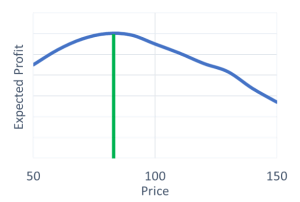
Measuring the relationship between price and P(Win) or quantity sets up a classic economics problem that every economics student learns through college. “Find the price that maximizes the expected profit.” Expected profit in my client’s case is simply profit from the project times the P(Win). However, for our client, and most firms in the real world, there exist extra constraints to consider such as regulatory restrictions, reputation damage, and relationship to other projects in the portfolio.

Figure 1: Illustration of classic price optimization problem.

Modeling Constraints and Optimizing Prices for the Entire Portfolio of Projects

Like many firms in the manufacturing industry, our client cannot rapidly increase production based on short-term increases in market demand. It takes significant investments in capital and human labor to expand their capacity. Simply optimizing each price for each quote, as illustrated in Figure 1, may lead to issues of overcapacity.

While having “too much” business is a good problem to have, in our client’s case it would lead to increased labor costs as they are forced to pay for overtime and may incur longer timescales for delivery which would hurt their reputation and lead to less revenue in the future.

To account for this, we not only had to consider the direct cost of a project but also the opportunity cost of a project. Different projects can have different margins. We wanted to use pricing as a tool to ensure our client’s limited capacity would be filled with the most profitable projects first and then filled up with the less profitable projects to fill up the remaining capacity.

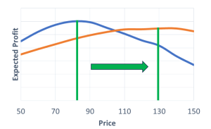
Taking the opportunity cost into consideration, can affect what the optimal price should be for a project. If a project is less profitable than most others in a portfolio, then the optimal price will shift to the right compared to what it should be when measured in isolation. (Figure 2).

Figure 2: Optimal price with and without opportunity cost. Note this chart is purely for illustrative purposes and was not based on actual data from our client.

Ends Results and Applications for Other Organizations

Near the beginning of this year, this client contacted HDR to inform us of how satisfied they were with the models we developed and their performance. The client estimated optimization models had increased their margins by 48% and “tripled their operating income in 2023.” This resulted in a very high ROI on hiring HDR.

As impressive as these results were from this client, they are certainly not unique. Time and time again, we have found that quantifying all aspects of important decisions leads to different decisions being made and, ultimately, better financial outcomes It is not uncommon for us to see the models we develop for our clients cause them to make different decisions or prioritize different measurements that end up saving or earning them a magnitude more than the amount they hired us for.

Some of the projects and methods used with this client we routinely use for projects involving cybersecurity, enterprise risk, military fuel costs, goodwill investments, ESG factors, and many others. If your organization is having difficulty quantifying essential items that affect your decision-making, please feel free to contact us.

Calibrating Chat GPT for Its Overconfidence

by Robert Weant | Nov 20, 2023 | Facilitating Calibrated Estimates

In a previous article, we measured how calibrated Chat GPT 4 was at providing a 90% confidence interval. During the experiment, after explaining what is meant by a 90% confidence interval, Chat GPT would provide a stated 90% interval that would only contain the actual answer 60% of the time. For comparison, on average humans’ performance is at 52% (This metric is slightly updated due to a larger sample size since the previous article was written). Thankfully, providing calibrated probability estimates is not some innate talent determined by genetics nor a skill bestowed upon people by the Gods of statistics. It is a skill that can be taught and learned.

Calibration Training: Understanding One’s Own Uncertainty

HDR has built upon decades of research in this area through the works of Nobel Prize winner Daniel Kahneman and political scientist Phillip Tetlock, to build the most comprehensive online calibration training platform available. Through a series of tests and training videos, humans learn how under or overconfident they are when giving probabilistic estimates and strategies that help them give more accurate probability assessments. When used correctly these strategies help humans translate their uncertainty into quantitative terms.

We put Chat GPT 4 through a similar process. Using 62 events that occurred after its data cut-off point, we went through several rounds of forecasting with Chat GPT where we asked it to provide 90% confidence interval estimates on topics such as sports, economics, politics, and pop culture. We then followed up by teaching it the same subjective forecasting strategies we teach humans in our training.

Below are the results of teaching these methods to humans and Chat GPT and recording their performance. For humans, these strategies were taught sequentially in which humans received a series of 6 tests and had their performance recorded. For Chat GPT, two sessions were created in which the temperature was set to 0 to decrease “creativity” in responses or as some might describe it “noise”. One was given a simple explanation of 90% confidence intervals and asked to forecast 62 events, the other was asked to apply the strategies mentioned above when forecasting the same 62 events.

	Initial Performance	After Training and Strategies
Humans	52% (10K intervals, 1001 humans)	78% (52K intervals, 1001 humans)
Chat GPT 4	64.5% (62 intervals, 1 session)	58% (62 intervals, 1 session)

When it comes to humans, teaching these strategies significantly improves calibration. While still not perfectly calibrated to a 90% level, after going through calibration training their overconfidence is greatly diminished. It is worth noting, that the average for humans is brought down by outliers. Essentially individuals, whom we suspect based on their recorded time to completion, quickly answer questions without reading them.

Chat GPT on the other hand, struggles to use these strategies effectively and gives slightly worse estimates. A closer examination reveals that the version that was taught the strategies starts with a much more narrow range, then sequentially widens the range, by small amounts on both ends. It did not discriminate between different questions and would modify its range by similar amounts for each forecast. The result is a range with a width closer to that of the other session. Fortunately, there is another way of calibrating Chat GPT.

Calibration Training Hard Calculated Adjustment

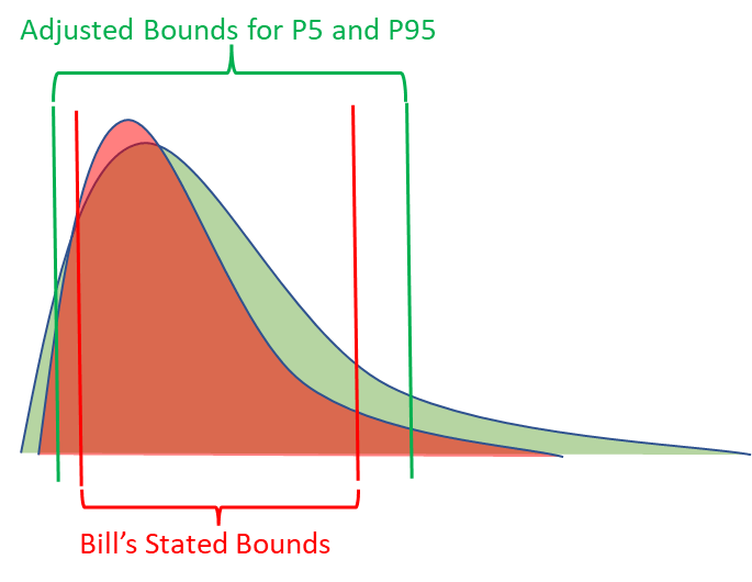
Anytime a human goes through calibration training, we know how to get calibrated 90% confidence intervals from them, even if they perform poorly during the calibration process. If Bill consistently gets 80% of the answers between his stated bounds, we know what metrics should be applied to his stated bounds in order to turn them into calibrated P5s and P95s. In other words, we know how to adjust for Bill’s overconfidence.

The exact same process can be applied to Chat GPT or other language models. To test this, we divided the set of 62 forecasts into a train and test set, with 31 forecasts in each. We calculated what the average adjustment would need to be for both the lower and upper bounds to be 90% calibrated for only the training set of questions. Then applied these adjustments to the test set of questions.

	Initial Stated Bounds	After Applying Adjustment
Train Set	68% (31 intervals)	90.3%
Test Set	61% (31 intervals)	87.1%

(Adjustments are calculated by normalizing the data on a scale of 0 to 1 with 0 = stated LB and 1 = stated UB)

This process was repeated 1000 times with different random samplings for the train and test data sets. After applying the adjustments developed from the training data sets, the average percent correct for the test data set bounds was 89.3%, which is nearly perfectly calibrated.

Practical Applications

Now that we have a method to obtain calibrated 90% confidence intervals from Chat GPT, can we use it to replace analysts’ subjective judgment when making decisions? Not exactly. The subjective confidence intervals given by Chat GPT should be viewed as initial baseline estimates. While calibrated to a 90% level, the intervals are much wider than what we would expect experts to provide. The information value Chat GPT has on a certain forecast is less than what we would expect from an expert on that topic.

For example, one of the forecasting questions was estimating Microsoft’s total 2022 revenue. After applying the adjustments to calibrate it, the output was a very wide range of $87 – 369 billion. I’m not a financial analyst with a focus on the tech industry, but I imagine obtaining a similar calibrated subjective forecast from financial analysts in January 2022 (Chat GPT’s data cut-off date) would result in a much more narrow range.

	Adjusted LB (P5)	Adjusted UB (P95)	Actual Answer
Microsoft Total 2022 Revenue	$86.7 Billion	$379.2 Billion	$198.3 Billion

The advantage Chat GPT and other generative AIs have is their speed and cost. In many models HDR builds for clients to help them make multi-million or even billion-dollar decisions, we’ll have a list of hundreds of variables that our client knows have an impact on the decision, but they are unsure how to quantitatively define them or who they should get to estimate them. It can take weeks to obtain estimates from experts or to collect data from other departments, while Chat GPT will take less than 5 minutes.

The key usefulness of starting with a calibrated baseline estimate is the implications of calculating the expected value of perfect information (EVPI). In every model we build, we calculate what the EVPI is for every variable. The EVPI is a monetized sensitivity analysis that computes how valuable it would be to eliminate uncertainty for a certain variable. It allows the analysts to pinpoint exactly how much effort they should spend analyzing certain variables. But this only works if there are initial calibrated estimates in the model.

In a follow-up article, I will be reviewing how HDR is incorporating Chat GPT in its decision models. This will include how we are utilizing it to estimate 90% confidence intervals within the model, how it can be prompted to build cashflow statements, and the implications of auto-generated EVPIs for follow-up analysis.

NOTE: Open AI released a major update for Chat GPT on November 6th. During this update, the data cut-off date was changed to April 2023. All interactions with Chat GPT mentioned in this article occurred in September and October of this year when the data-cutoff point was still January 2022 for Chat GPT 4.

Is ChatGPT as Overconfident as Humans?

by Robert Weant | Sep 12, 2023 | Facilitating Calibrated Estimates

“It’s not what we don’t know that hurts, it’s what we know for sure that just ain’t so.”

The quote above is often attributed to Mark Twain. Ironically, the authorship of this quote being somewhat uncertain, beautifully illustrates the very point it makes. Nevertheless, the quote accurately describes the dangers of humans being overconfident. Put into quantitative terms, being overconfident is assigning higher probabilities to items than what should be the case. For example, if I’m asked to give a 90% confidence interval for 100 questions, the correct answers should be between my stated bounds 90% of the time. If it is less than 90%, I’m overconfident, and if it’s more than 90% I’m underconfident.

There have been many peer-reviewed papers on this topic that reveal humans, regardless of field or expertise, are broadly overconfident in providing probabilistic estimates. Data collected by HDR on calibration performance supports this conclusion. When participants prior to any sort of training were asked to provide 90% confidence intervals for a set of questions, on average, only 55% of answers fell within their stated ranges.

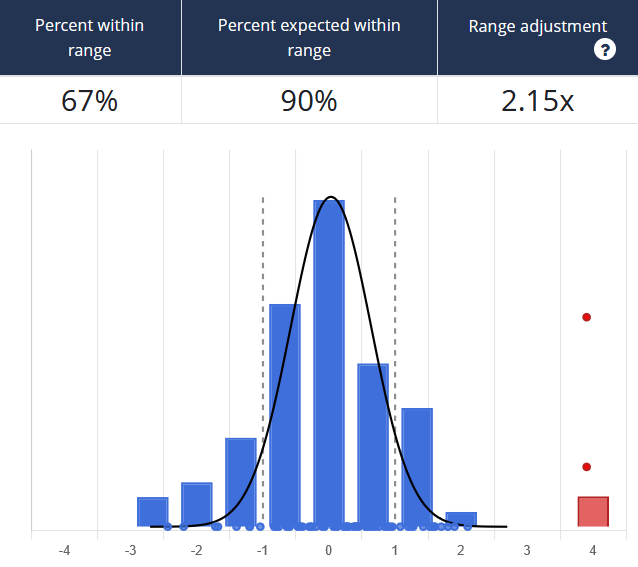
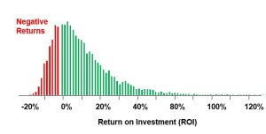
An example from our Calibration Training shows a group only getting 67% of questions within their stated ranges. Here the estimators’ lower and upper bound responses are normalized as values between -1 and 1. If the correct answer is outside their range, it falls above or below -1 and 1 on the graph. The red dots represent outliers where the response wasn’t just wrong but considerably far off.

So how does AI stack up against humans here? In order to compare the performance of AI relative to human estimators, we asked 18 instances of ChatGPT 4 to provide 90% confidence interval estimates for a set of 20 questions on topics of sports, economics, and other metrics that are easily verifiable. This resulted in a total of 360 unique estimates. This differed from the trivia questions we use when calibrating human experts as ChatGPT 4 has access to all that information. Remember, the goal of calibration is not to answer questions correctly but to accurately reflect one’s own uncertainty. Trivia questions are used in our training because immediate feedback can be provided to individuals, which is essential in improving performance. To replicate this effect with AI, we limited the questions to ones that had actual answers manifest sometime between September 2021 (the data cutoff point for ChatGPT) and August 2023. An example of such a question is “How much will the top-grossing film earn internationally at the box office in 2022?”. This way we could evaluate whether the actual value (when analyzed retrospectively) fell within the estimated bounds by ChatGPT 4.

The results indicated below show the average calibration of the ChatGPT instance to be 60.28%, well below the 90% level to be considered calibrated. Interestingly, this is just slightly better than the average for humans. If ranked amongst humans, ChatGPT 4’s performance would rank at the 60th percentile from our sample.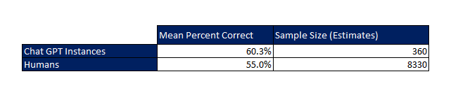

If we applied this average level of human overconfidence toward hypothetical real-world cases, we would drastically underestimate the likelihood of extreme scenarios. For example, if a cybersecurity expert estimated financial losses to be between $10 – $50 million when a data breach occurs, they are stating there is only a 5% chance of losing more than $50 million. However, if they are as overconfident as the average human, the actual probability would be closer to 22.5%.

As far as humans go, there is some good news. Being accurately calibrated is not some innate talent determined by genetics, but a skill that can be taught and improved upon. Papers and studies provide conclusive evidence that humans can greatly improve their ability to give probabilistic estimates. HDR built upon these studies and developed online training that is specifically designed to improve individual human calibration for probabilistic estimates. Before training the average calibration level was 55% when trying to provide a 90% confidence interval for an uncertain quantity. By the end of training, this improved to 85%. Humans were able to better understand their own uncertainty and translate it into useful quantitative terms.

As we begin to rely more on language models, it is essential that we understand the uncertainty in the output they produce. In a follow-up and more in-depth study, HDR will be testing to see whether we can train ChatGPT and other language models to assess probabilistic estimates more accurately, and not fall victim to overconfidence or as Twain might put it “thinking what we know for sure that just ain’t so.”

Find out more about our state-of-the-art Calibration Training here

A Quant’s Approach to Buying vs Renting

by Robert Weant | Aug 8, 2023 | How To Measure Anything Blogs, Personal Finance

Tab 1…., Tab 2…., Tab 1.., Tab 2. I was anxiously clicking back and forth between two tabs on Zillow.com for the DC area. One shows the “For Sale” homes in a popular young professional neighborhood, and the other “For Rent” in the same area. Two nearly identical townhouse apartments were on the market, one for a selling price of $375K and the other listed for rent at $1,995 per month. When Googled “Is it better to buy or rent” the results give everyone’s opinion from self-proclaimed financial gurus prophesizing the common adage “Renting is for Suckers” to van living pseudo-philosophers who subscribe to the belief that “You don’t want to be tied down to one place man.” Even Chat-GPT gives me a very ambivalent answer stating, “The decision between buying and renting is complex and depends on many uncertain factors”. Fortunately, the company I work for Hubbard Decision Research (HDR), specializes in making decisions given many uncertain factors. Applied Information Economics (AIE), developed by HDR’s founder Douglas Hubbard, provides a practical statistical framework for making this decision or others with high degrees of uncertainty. It employs methods proven by a large body of peer-reviewed academic research and empirical evidence on improving human expert judgments. As a management consulting firm, we are routinely hired by some of the world’s largest companies and government organizations to apply this framework to large difficult decisions. The same framework can be applied to personal financial decisions in a 4-step process. 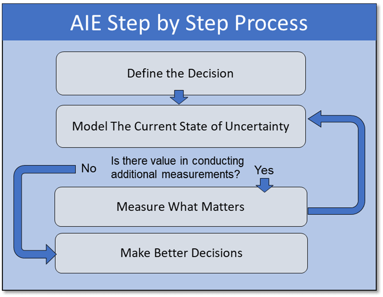Step 1: Define the Decision Should I buy or rent an apartment? Given that I don’t have any personal preference for homeownership itself, which decision is more likely to lead to a better financial outcome? Step 2: Model What We Know Now To model this decision, a Monte Carlo simulation was used to generate 1,000 different possible scenarios based on defined probability distributions for the variables that influence the decision. This may sound complicated at first glance. References to simulations bring up mental images of the Matrix or Dr. Strange using the Time Stone to see 14 million different simulations and only one way to defeat Thanos. But when explained, it’s quite straightforward. Rather than using a fixed value for a variable I’m unsure about such as “Time until reselling of home”, I use a range with a confidence interval. I’m not sure how long I would potentially live in the apartment, but I’m 90% sure it would be between 3-15 years. While I may not possess an infinity stone to see all these simulations, I do possess a tool equally as powerful for practical decision-making: Excel. In Excel, standard cashflow models were built to show how my financial inflows and outflows would compare if I rented or bought one of the apartments, and the net present value (NPV) of the difference was calculated. 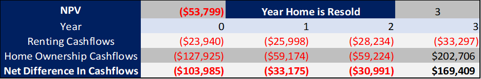These cashflows were calculated based on 17 different variables that have an impact on the decision. For variables, I am uncertain about, the model randomly samples from a confidence interval provided. The Model repeats this 1000 times and records the Simulated Value, and Cashflows for each simulation. Based on the recorded simulated values and cashflows, the model generates a probability distribution for possible NPVs, which will suggest an informed decision. If the expected NPV (average NPV across all situations) is positive, the decision should be to buy; if it is negative, the decision should be to rent. 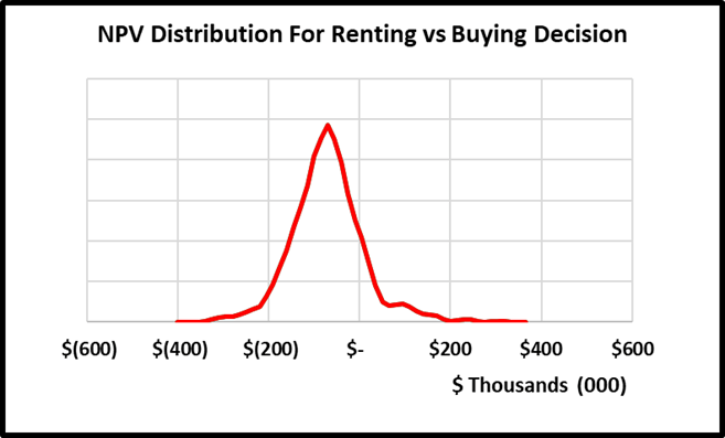The big caveat is this is based on a probability-weighted outcome, and there is a chance the model suggests the wrong decision. However, there are ways to reduce this probability by conducting additional measurements. Step 3: Measure What Matters: One of the benefits of using Monte Carlo simulations versus deterministic models with fixed values is that we can calculate the expected value of perfect information (EVPI). It is how much a person should be willing to pay to eliminate their uncertainty about a variable. The calculation is essentially the probability of being wrong multiplied by the cost of being wrong. 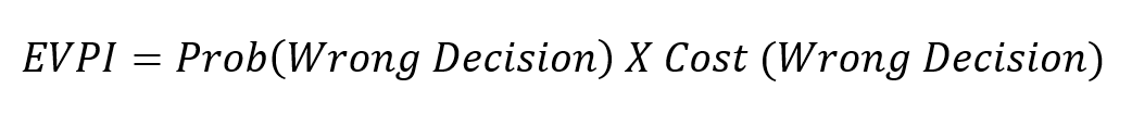By measuring and ranking EVPIs, we obtain a practical list of the most important uncertain variables to spend time measuring or conducting additional analysis on. If initially, I’m unsure what my mortgage rate would be and give a 90% confidence range of between 4-9%, the maximum I would be willing to pay a bank to give me a precise mortgage quote guarantee would be the EVPI. In this case $1,407. The cost for me of spending 15 minutes to get an online mortgage quote is well below this EVPI value. After doing so, I received a quote of 6.7%. Replacing this range with the fixed value and rerunning the model results in a narrower distribution of NPVs as seen below and thus reducing my uncertainty about the decision. 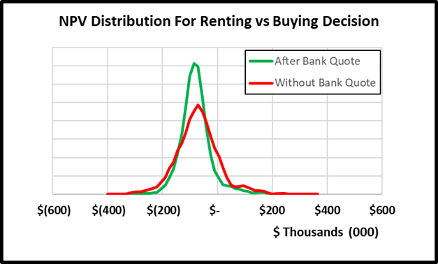Changing the mortgage rate from a range to a constant also changes the EVPIs of other variables. While in the original model, I had 4 variables with EVPI values, the updated model shows the only variable worth conducting additional measurement on is the estimated annual increases in home prices over the period of ownership. Unfortunately for me, I do not have a magic crystal ball, nor an oracle I can con pay to tell me precisely what home prices will do in the future. I could spend hours researching the market mechanisms of home price increases to come up with narrower range estimates for the lower and upper bounds. However, based on the EVPI, I do not think the slight reduction in uncertainty is worth it. I can confidently move on to making my decision. Step 4: Make Better Decisions: The final model results show the expected value of buying versus renting the apartment is $-79,072. In 93.8% of the simulations, I would be better off renting the apartment vs buying the apartment. This conclusion could change as new information becomes available and if mortgage rates start to decrease, but for now I can very confidently make the decision that I’m financially better off renting than buying. Other Applications of AIE: This was a simple example of how Applied Information Economics can improve personal financial decisions. The same steps can be applied to practical large-scale business investments. At Hubbard Decision Research, we routinely apply the same step-by-step process to multi-million or even multi-billion-dollar decisions. We also provide training to improve our client’s ability to quantify anything, build probabilistic models, and not only make better decisions but make better decision-makers. For more information, explore the rest of the website or contact us at info@hubbardresearch.com.